Probability distributions

Table of contents:
How to start?
If you check from the Wikipedia you may find good results:
One other resource is scipy.
| Distributions | Comment |
|---|---|
| beta(a, b[, size]) | Draw samples from a Beta distribution. |
| binomial(n, p[, size]) | Draw samples from a binomial distribution. |
| chisquare(df[, size]) | Draw samples from a chi-square distribution. |
| dirichlet(alpha[, size]) | Draw samples from the Dirichlet distribution. |
| exponential([scale, size]) | Draw samples from an exponential distribution. |
| f(dfnum, dfden[, size]) | Draw samples from an F distribution. |
| gamma(shape[, scale, size]) | Draw samples from a Gamma distribution. |
| geometric(p[, size]) | Draw samples from the geometric distribution. |
| gumbel([loc, scale, size]) | Draw samples from a Gumbel distribution. |
| hypergeometric(ngood, nbad, nsample[, size]) | Draw samples from a Hypergeometric distribution. |
| laplace([loc, scale, size]) | Draw samples from the Laplace or double exponential distribution with specified location (or mean) and scale (decay). |
| logistic([loc, scale, size]) | Draw samples from a logistic distribution. |
| lognormal([mean, sigma, size]) | Draw samples from a log-normal distribution. |
| logseries(p[, size]) | Draw samples from a logarithmic series distribution. |
| multinomial(n, pvals[, size]) | Draw samples from a multinomial distribution. |
| multivariate_normal(mean, cov[, size, …) | Draw random samples from a multivariate normal distribution. |
| negative_binomial(n, p[, size]) | Draw samples from a negative binomial distribution. |
| noncentral_chisquare(df, nonc[, size]) | Draw samples from a noncentral chi-square distribution. |
| noncentral_f(dfnum, dfden, nonc[, size]) | Draw samples from the noncentral F distribution. |
| normal([loc, scale, size]) | Draw random samples from a normal (Gaussian) distribution. |
| pareto(a[, size]) | Draw samples from a Pareto II or Lomax distribution with specified shape. |
| poisson([lam, size]) | Draw samples from a Poisson distribution. |
| power(a[, size]) | Draws samples in [0, 1] from a power distribution with positive exponent a - 1. |
| rayleigh([scale, size]) | Draw samples from a Rayleigh distribution. |
| standard_cauchy([size]) | Draw samples from a standard Cauchy distribution with mode = 0. |
| standard_exponential([size]) | Draw samples from the standard exponential distribution. |
| standard_gamma(shape[, size]) | Draw samples from a standard Gamma distribution. |
| standard_normal([size]) | Draw samples from a standard Normal distribution (mean=0, stdev=1). |
| standard_t(df[, size]) | Draw samples from a standard Student’s t distribution with df degrees of freedom. |
| triangular(left, mode, right[, size]) | Draw samples from the triangular distribution over the interval [left, right]. |
| uniform([low, high, size]) | Draw samples from a uniform distribution. |
| vonmises(mu, kappa[, size]) | Draw samples from a von Mises distribution. |
| wald(mean, scale[, size]) | Draw samples from a Wald, or inverse Gaussian, distribution. |
| weibull(a[, size]) | Draw samples from a Weibull distribution. |
| zipf(a[, size]) | Draw samples from a Zipf distribution. |
Random variable
For each distribution there is a generator function. In statistics and probability theory there is a term called random variable.
This random variable (sometimes random quantity or stochastic variable) is associated with some random phenomenon. Random variable takes values based on on that phenomenon.
Once we have a random variable, we can understand the probability distribution based on the PDF (Probability Density Function) and Cumulative Distribution Function (CDF).
We can also analyse Inverse Cumulative Distribution Function or Quantile function.
We can also specify set probability distribution using the moment-generating function of a real-valued random variable.
The Cauchy distribution has no moment generating function.
Division of distributions
I would like to outline these simple distribution types.
First, based on the data type:
- Continuos
- Discrete
Then based on the number of features:
- Univariate (single feature)
- Multivariate (multiple features)
- Bivariate (exactly two features)
Then, based on the distribution type:
- Uniform
- Normal
- Exponential
- Gamma
Continuos distributions
Uniform distribution
Example:
What is the range of values provided by random.random() in Python?
import random
random.random()
#0.6447902854472809
We can check and see all the values will be inside $[0, 1)$ range.
Example:
# distribucija random brojeva
import matplotlib.pyplot as plt
import random
import numpy as np
a100 = [random.randint(0, 100) for p in range(0, 100000)]
a50 = [e for e in a if e<50]
fig,ax=plt.subplots(dpi=153)
# counts, bins = np.histogram(a100)
ax.hist(a100, bins=10, color=['r'])
ax.hist(a50, bins=10, color=['#ffffff66'], histtype='step' )
ax.title.set_text('Uniform distribution')
ax.set_ylabel('Number of elements')
ax.set_xlabel('10 beans')
plt.show()
Output:
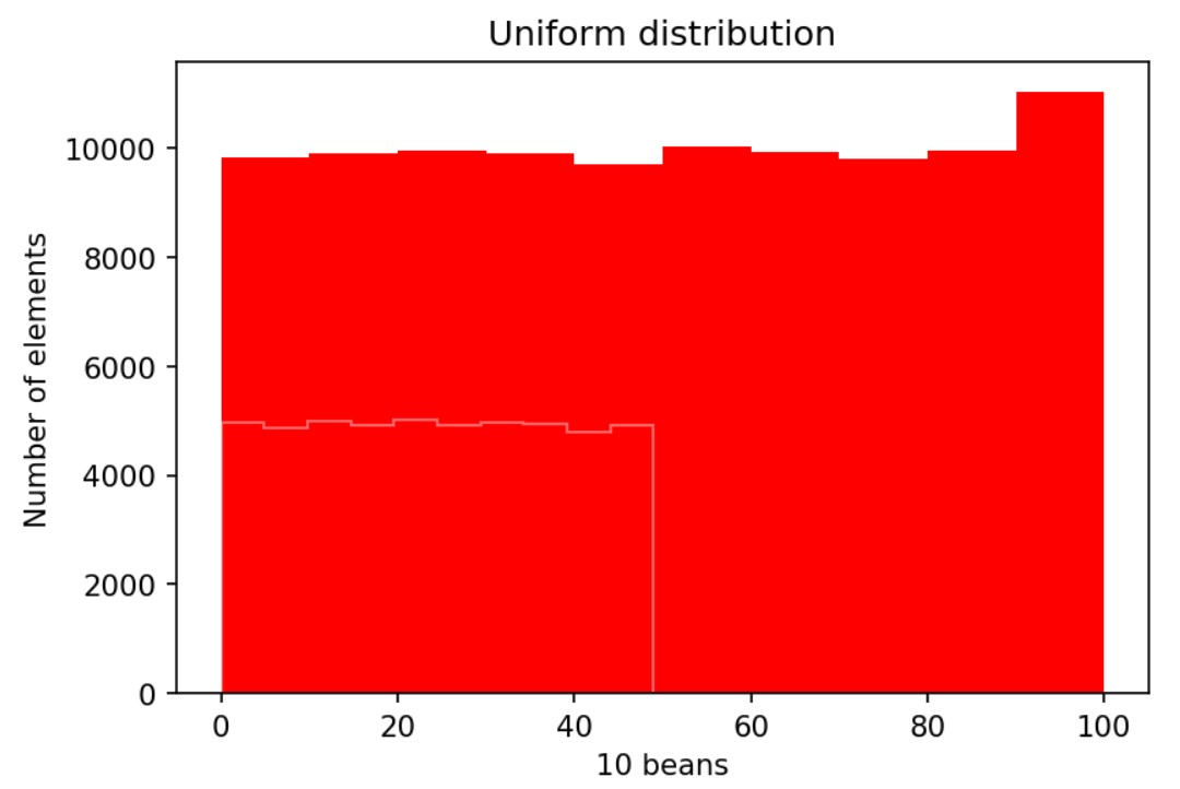
We have 10 bins for the arrays a100 and a50. The y axis denotes the number of elements, and the x axis denotes the 10 beans.
Uniform distribution means flat at the top. For the random numbers we expect the uniform distribution.
Normal distribution
This is continuos distribution. For the list of other continuos distributions check https://docs.scipy.org/doc/scipy-0.16.0/reference/stats.html
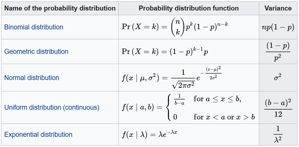
From Wikipedia you may see the normal distribution PDF:
$PDF: f(x)=\frac { e^{\small -\frac 12 ({ x- \mu \over \sigma} )^2}} {\sigma \sqrt{2\pi}}$
or, when $\sigma=1$, and $\mu=0:$
$PDF: f(x)=\frac{\large e^{\frac{\small x^2}{2} }}{\sqrt{2\pi}}$
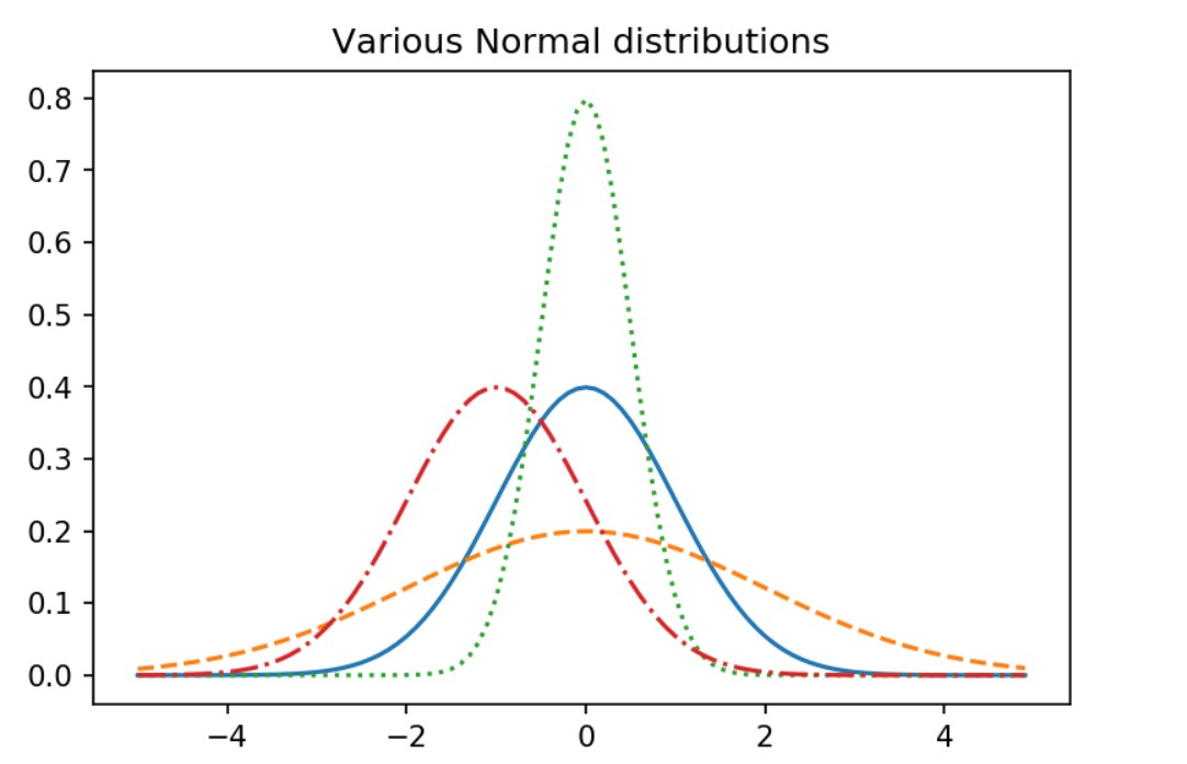
Let’s implement this in Python:
import math
from matplotlib import pyplot as plt
def normal_pdf(x, mu=0, sigma=1):
    sqrt_two_pi = math.sqrt(2 * math.pi)
    return (math.exp(-(x-mu) ** 2 / 2 / sigma ** 2) / (sqrt_two_pi * sigma))

xs = [x / 10.0 for x in range(-50, 50)]
fig,ax = plt.subplots(dpi=153)
ax.plot(xs,[normal_pdf(x,sigma=1) for x in xs],'-',label='mu=0,sigma=1')
ax.plot(xs,[normal_pdf(x,sigma=2) for x in xs],'--',label='mu=0,sigma=2')
ax.plot(xs,[normal_pdf(x,sigma=0.5) for x in xs],':',label='mu=0,sigma=0.5')
ax.plot(xs,[normal_pdf(x,mu=-1) for x in xs],'-.',label='mu=-1,sigma=1')
ax.title.set_text("Various Normal distributions")
plt.show()
scipy.stats.norm gives us parameters such as loc and scale. It also has a variety of methods and we explored rvs, cdf, sf, ppf, interval, and isf in this article.
Matplotlib gives us easy and extensive tools to change details of a figure including 3D.
Discrete distributions
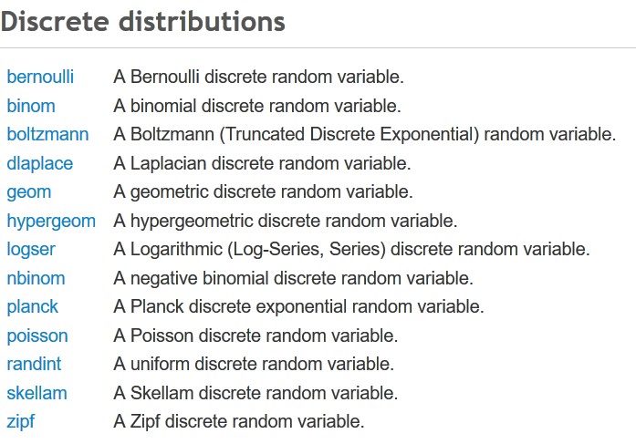
The previous list is what I found for Python scipy library.
We should mention the randint, random number generator. This is the same as random.randint from import random uniform distribution.
Then if we analyse the Bernoulli trials (or binomial trials) with exactly two possible outcomes success and failure for the experiment.
For Bernoulli trials probability of success is the same each time we conduct our experiments. This means probability of failure is also always the same as these two probabilities should add to 1.
We find this trials when flipping a coin. Head is success and tail is the failure.
To describe the number of heads after n trials, we use binom distribution or binomial discrete distribution.
For exactly the same coin flipping problem geometric distribution geom in scipy is used to represent the number of failures before the first success.
Negative binomial distribution nbinom is used to represent the number of failures before the x-th success.
Bernoulli discrete random variable is for Bernoulli distribution which is a special case of binomial distribution where $n=1$, just for a single trial.
Poisson distribution, poisson in scipy is used to represent the number of events in a period of time. It may be used for predicting computer clicks.
…
tags: probability & category: math