Notation:

Predictors or covariates or features are columns with the data. You don’t predict them, but you use them to predict. They are also called independent variables.

The predictant: the column(s) you predict. Sometimes called outcome variable or dependent variable.

Table of contents:

• Example Linear Regression
• Multilayer perceptrons regression vs. ordinary least squares (OLS) linear regression (statistical approach).
• Logistic regression
  • How to deal with missing values?
• Linear regression
  • How to deal with missing values and outliers?
  • Rule of 22
• Removing outliers procedure
  • Rule of thumb to detect outliers
  • Removing contextual outliers

Example Linear Regression

Let’s start with an example. We will use numpy and matplotlib together with scikit-learn for LinearRegression evaluation.

import numpy as np
from matplotlib import pyplot as plt

# function for the target y = f(x)
def f(x):
    return 2*x+3

# we will use linear regression to find coefficients 2 and 3
n = 1000  # number of samples

x = np.linspace(-10, 10, n) # feature
y = f(x)+np.random.normal(scale=5,size=n)
print(x.shape, y.shape)

lreg = LinearRegression()
lreg.fit(x.reshape(-1, 1), y)
print(lreg.coef_) # should be 2
print(lreg.intercept_) # should be 3
p = lreg.predict(x.reshape(n,1))
fig,ax=plt.subplots(figsize = (9,6), dpi=103)

ax.title.set_text('Linear Regression')
ax.scatter(x,y,c='g')
ax.plot(x,p,c='b') # prediction
plt.show()

Output:

(1000,) (1000,)
[2.00846018]
3.0270821698099404

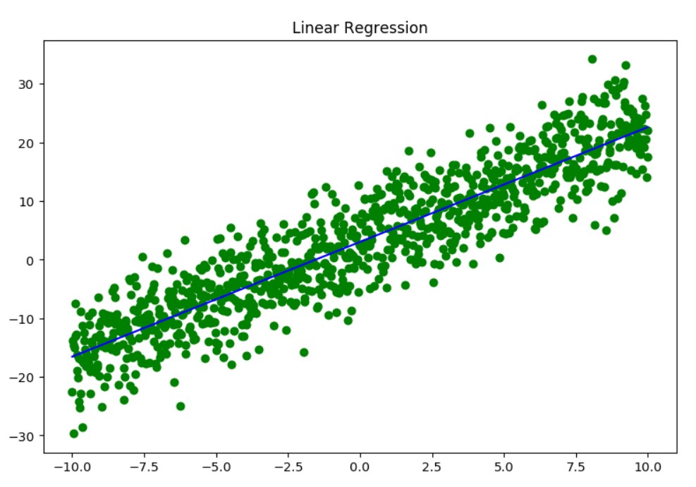
From 1000 green scatter points we created the prediction - the blue line.

The lreg.coef_ value is close to 2 and lreg.intercept_ is close to 3 as we expected.

Multilayer perceptrons regression vs. ordinary least squares (OLS) linear regression (statistical approach).

Multilayer perceptrons or deep neural networks predictions should improve over least square linear regression.

Deep neural networks are capable is to learn more thanks to nonlinearities they use.

In that respect you may say deep neural networks improve linear regression prediction.

Our first example would represent statistical linear regression approach.

We found $c_0$ and $c_1$ coefficients for the $y=c_0+c_1\cdot x$.

In case we have multiple features we would have:

$y_i=c_0+c_1\cdot x_i$

Logistic regression

Logistic regression in machine learning you typically use to estimate categorical target.

Don’t be confused with the name, logistic regression is used for classification.

All your features need to be numeric. They contain values that describe the target’s class.

In pandas you convert strings to integers in order to achieve that, in scikit-learn you create labels maybe using LabelEncoder.

Logistic regression in addition to predicting the class of observations in your target variable, it indicates the probability for each estimate.

It is important to note we do not request to have linear relation between the features and the target.

The features are all the columns we have in our database except the target column we predict.

Target feature distribution may be any, not necessary normal distribution.

Logistic regression can predict multiple features, but all these features should be mutually independent.

How to deal with missing values?

Just remove the missing values.

Linear regression

If you just use a single feature to predict this will be easy as: \(y=c_0 + c_1 x\)

If we use multiple columns this is often called multiple linear regression.

Linear regression only works with numerical variables. This means you need to do conversions on your dataset first before applying.

Conversion assumes you analyse the cardinality of your categorical variables and replace them with numerical corresponds.

How to deal with missing values and outliers?

Fix the missing values. Sometimes you may need to remove observations from you dataset.

Remove the outliers, else you may have wrong predictions.

Linear regression assumes all features are independent, so you need to remove dependent variables.

Once you fit, there need to be a linear relationship between the dataset features and the target variable.

If this is not the case try using a log transformation to compensate.

Rule of 22

You should have at least 22 observations per predictive feature if you expect to generate reliable results using linear regression.

Removing outliers procedure

Removing outliers is applicable not just for the regression problems, but for all machine learning problems.

Outliers are data different than the majority of data. Frequent we ignore them, but some methods require to remove outliers from our dataset.

Outliers are often caused by some measuring errors and give bad feedback for our data analysis. They may provide wrong idea about the mean of our data, which further brings wrong idea about the deviations (standard and absolute).

This again lead to wrong correlations among the features.

Machine learning and statistical models actually assume your data is free of outliers.

Detecting outliers is very important. This assumes spotting the anomalies, hardware failures, saving values out of the expected ranges (distributions), different hacks and attacks.

There are several categories of outliers:

• data not in a normal range of values for a feature (weight of an elephant is 200 gr)
• contextual outliers ( 3 years old kids height is 180cm )
• collective outliers (all equipment older that 1950 are set to be from year 1950 )

Most of the methods to detect outliers are very simple:

• 25 and 75 percentiles bound
• 3 sigma bounds

The IQR (Inter Quartile Range) means just detecting the Q1 (25%) and Q3 (75%) values, and potentially remove anything else.

Rule of thumb to detect outliers

Find the range [Q1-1.5 * IQR, Q3+1.5 * IQR].

If the minimum value is less the range or max is greater that the range the variable probably has outliers.

Removing contextual outliers

To remove contextual outliers we need to considering multiple variables at the same time. There are many methods for just that:

• scatter-plot matrix
• Boxplot
• Density-based spatial clustering
• PCA