How to prevent the overfitting | Regularization

Table of Contents:

• Detecting overfitting
• General division of regularization techniques
  • 1. Regularization based on data
    • Data augmentation
    • Cross-validation
    • Dropout
    • Batch norm
    • Large Batch size
    • Half precision
  • 2. Regularization based on network architecture methods
    • Bagging
    • Boosting
    • Stacking
  • 3. Regularization based on error function methods
  • 4. Regularization term $R$ methods
    • L1 regularization
    • L2 regularization
    • Early stopping
  • 5. Regularization based on optimization function $arg \ min$

Machine learning engineers are afraid of overfitting.

First they detect overfitting and then they try to avoid it. Here are the common techniques to prevent overfitting.

Detecting overfitting

Once we have a train and test datasets we evaluate our model against the train and against the test datasets.

Depending of our metrics, we may find out:

• validation loss » training loss: overfitting
• validation loss > training loss: some overfitting
• validation loss < training loss: some underfitting
• validation loss « training loss: underfitting

If validation loss is much bigger than the training loss we call it overfitting.

Our aim is to make the validation loss as low as possible. Some overfitting is nearly always a good thing. All that matters in the end is: the validation loss as low as you can get it.

Regularization is any technique that aims at making the model generalize better, that produces better results on the test set.

General division of regularization techniques

We know neural network is a function:

$f_{w}: x \mapsto y$, where $w \in W$ are trainable weights.

Training the network means finding a weights by minimizing the objective (loss) function $\mathcal{L}: W \rightarrow \mathbb{R}$ as follows:

\[w^{*}=\underset{w}{\arg \min } \mathcal \ {L}(w)\]

We can express the loss function as the expected risk:

\[\mathcal{L}=\mathbb{E}_{(x, t) \sim P}\left[E\left(f_{w}(x), t\right)+R(\ldots)\right]\]

Where:

• $E$ is the error function
• $R$ is the regularizer part
• $t$ are targets

We don’t know the data distribution $P$ in the general case, but we know the data set $\mathcal D$.

So the expected risk is:

\[\underset{w}{\arg \min } \frac{1}{|\mathcal{D}|} \sum_{\left(x_{i}, t_{i}\right) \in \mathcal{D}} E\left(f_{w}\left(x_{i}\right), t_{i}\right)+R(\ldots)\]

Now we know the formal background to divide the regularization methods.

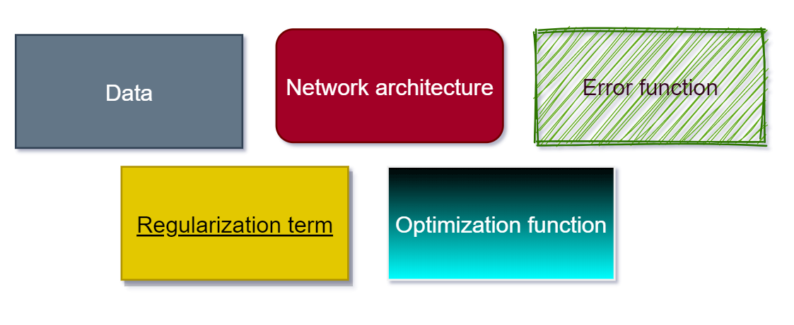
Regularization can be based:

1. on data $\mathcal D$
2. on the network architecture $f$
3. error function $E$
4. regularization term $R$
5. optimization function $arg \ min$

Here we review all these:

1. Regularization based on data

Data augmentation

Data augmentation’s simple idea is to train with more data. There are some problems with this approach in many cases, because you may not have the data, or you can get it but it is very expensive, time consuming.

This is why you may try to make some transformations on the data if this is possible. This works for images, simple image flip for instance.

A way around the problem may be to generate the probability distribution fist (i.e. GANs), and then to generate new unseen data from this distribution.

Cross-validation

Cross-validation idea is this:

• use training data to generate a split
• each split has training and validation parts

If we instead just one split (two parts), create k parts we call it k-fold cross-validation

This means we have data into k subsets, called folds. Then, we train the algorithm on k-1 folds while using the remaining fold as the test set.

The test set is called the holdout.

Dropout

Dropout switches off some neurons in a layer so that they do not contribute any information or learn any information during forward step.

It works while training only.

There is $p$ probability to zero elements of the input tensor, defined by Bernoulli distribution. Based on Bernoulli distributions the outputs are scaled by $\frac{1}{1-p}$.

To explain dropout to a kid. Imagine classroom and all the time the same two kids answers the teacher’s questions. Teacher will ignore them for a while and ask other kids as well. Other kids may answer wrongly, but the teacher will correct them and this way the whole class learns better.

Batch norm

Batch norm is a network layer. The idea is to reshape the input distribution to a new distribution $\mathcal N(0, 1)$. This helps greatly to create deep network architectures. It effectively controls the data because the neuron activations should ideally be around 0 with the variance of 1.

Large Batch size

Using a larger batch size may add a regularization effect so in some cases you may even remove the dropout. A nice example may be found here.

Half precision

Converting a model to half precision for instance in PyTorch improves the regularization.

Few last regularization techniques we may add also to a section 2. Regularization based on network architecture.

2. Regularization based on network architecture methods

One common network architecture trick would be to use ensembles.

Ensembles are combined separate models. The most well known are:

• bagging ensembles
• boosting ensembles and
• stacked ensembles

Bagging

Well known bagging model is the random forest. This is an ensemble made from multiple decision trees so I will use the terms from that scope.

• we train some number of “strong” learners in parallel
• “strong” learners would be fully grown decision trees, deep with low bias, high variance
• each tree has a bit different train and validation data
• a strong learners are opinionated, individually they can learn items no other strong learner from ensemble can
• the final ensemble model will ignore learn items that are specific just to some trees and will promote those that are similar among the trees
• they can work both as classification and regression models.

Boosting

Boosting took a different approach.

• we train a large number of “weak” learners in sequence
• weak learners do have high bias, low variance
• weak learners could be trees where we limit the max deep
• each tree learns from the mistakes of the previous tree
• boosting then combines all the weak learners into a single strong learner.

Bagging and boosting approaches are different:

Boosting uses simple base models and tries to boost their aggregate complexity.

Bagging uses complex base models and tries to average their predictions.

Stacking

Stacking was invented in 1992 by Wolpert.

Stacking 4 steps:

• Create train and validation sets (splitting)
• Train based models on train set
• Predict using based models on validation set
• Stack predictions of base models to train high level models (meta models)

3. Regularization based on error function methods

The error function $E$ typical examples are mean squared error (regularization) or cross-entropy (classification).

Different error functions we select have a regularizing effect in comparison to others.

Error function is dependent on targets $t$.

4. Regularization term $R$ methods

$R$ is independent of targets. I will mention three types of regularization.

L1 regularization

A regression model that uses L1 regularization technique is sometimes called Lasso Regression.

L1 name is given by L1 weights vector norm which is a sum:

The loss function is this:

$\mathcal L = f(\hat y, y) + \lambda * \sum { \mid w \mid }$, where $\lambda$ is our constant.

L1 adds absolute weight penalties to the loss function. This in effect shrinks the less important features coefficient to zero (read: removes less important features).

It works well with models having a large (read: huge) number of features since it is made to ignore the less important features.

L2 regularization

Also called weight decay. The name was given by L2 norm of weights vector:

And the loss function is:

$\mathcal L = f(\hat y, y) + \lambda * \sum {w^2}$

Note the squared L2 norm at the end of the loss function (not actually the L2 norm).

Here $\lambda$ controls the importance of the regularization.

When learning a linear function $f$, characterized by an unknown vector $w$ such that $f(x)=w \cdot x$, one can add the L2-norm of the vector $w$ to the loss expression in order to prefer solutions with smaller norms.

Sometimes we may rewrite:

$\mathcal L = f(\hat y, y) + \frac{1}{2} \lambda * \sum {w^2}$

or

$\mathcal L = f(\hat y, y) + \frac{1}{2} \lambda * \sum {|w|_2^2}$

I believe the last notation should be used throughout the universe.

We add $\frac{1}{2}$ in front of lambda because the fist derivation will neglect it as the L2 norm is differentiable and can be used in GD.

Early stopping

This strategy is used to avoid the phenomenon called learning speed slow-down.

When the accuracy of the algorithm in one iteration stops improving after some point or even gets worse than we should stop and continue the next iteration. This is called early stopping.

Early stopping is time regularization.

Where the training procedure (usually gradient descent) learns complex functions with increasing iterations, we can control the model complexity and improve generalization if we regularize for time.

Early stopping implementation uses one data set for training, one statistically independent data set for validation and another for testing.

The model is trained until performance on the test set no longer improves and then applied to the validation set.

5. Regularization based on optimization function $arg \ min$

This basically means we should try different optimization functions as they may have different regularization effects depending on our problem.

---

Reference: 1. Regularization for Deep Learning: A Taxonomy (Jan Kukačka, Vladimir Golkov, and Daniel Cremers)

---