Python SciPy examples

SciPy is concise open-source library based on NumPy, Pandas, Matplotlib, SymPy. For more dependencies check out the official link
Table of contents:
Modules
SciPy contains modules for:
| Module | Description |
|---|---|
| scipy.cluster | Vector quantization / Kmeans |
| scipy.constants | Physical and mathematical constants |
| scipy.fftpack | Fourier transform |
| scipy.integrate | Integration routines |
| scipy.interpolate | Interpolation |
| scipy.io | Data input and output |
| scipy.linalg | Linear algebra routines |
| scipy.ndimage | n-dimensional image package |
| scipy.odr | Orthogonal distance regression |
| scipy.optimize | Optimization |
| scipy.signal | Signal processing |
| scipy.sparse | Sparse matrices |
| scipy.spatial | Spatial data structures and algorithms |
| scipy.special | Any special mathematical functions |
| scipy.stats | Statistics |
| … |
These are also called subpackages.
There is also a module called scipy.misc for various utilities that don’t have another home.
Basic Examples
Example:
from scipy import misc
import matplotlib.pyplot as plt
face = misc.face()
fig,ax=plt.subplots(dpi=153)
ax.set_axis_off()
ax.imshow(face)
plt.show()
Output:
Advanced Examples
Fitting a curve
In this example we start from scatter points trying to fit the points to a sinusoidal curve.
We know the test_func and parameters, a and b we will also discover.
x_data is a np.linespace and y_data is sinusoidal with some noise.
We will be using the scipy optimize.curve_fit function with the test function, two parameters, and x_data, and y_data forwarded as input.
from scipy import optimize
import matplotlib.pyplot as plt
x_data = np.linspace(-5, 5, num=50)
y_data = 2.9 * np.sin(1.5 * x_data) + np.random.normal(size=50)

fig, ax = plt.subplots(dpi=153)

def test_func(x, a, b):
    return a * np.sin(b * x)

params, params_covariance = optimize.curve_fit(test_func, x_data, y_data, p0=[2, 2])
print(params)
ax.scatter(x_data,y_data)
ax.plot(x_data, test_func(x_data,params[0], params[1]), c='r')
plt.show()
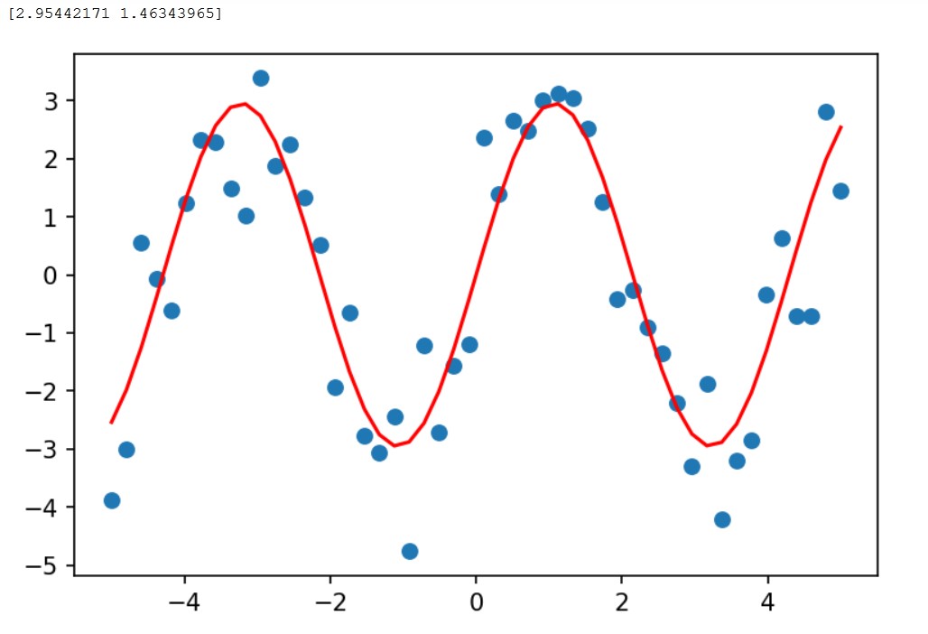
The red curve is what we will get, together with teh params we print.
Interpolation
Interpolation is another technique and in here we are using the interval [0,1] with 10 measurements (measured_time).
We also have the interpolation time with high resolution np.linspace(0, 1, 50).
import matplotlib.pyplot as plt
measured_time = np.linspace(0, 1, 10)
noise = (np.random.random(10)*2 - 1) * 1e-1
measures = np.sin(2 * np.pi * measured_time) + noise
fig, ax = plt.subplots(dpi=153)
ax.scatter(measured_time, measures) # Blue dots

# Interpolation time
from scipy.interpolate import interp1d
interpolation_time = np.linspace(0, 1, 50)
linear_interp = interp1d(measured_time, measures)
linear_results = linear_interp(interpolation_time)
cubic_interp = interp1d(measured_time, measures, kind='cubic')
cubic_results = cubic_interp(interpolation_time)

ax.plot(interpolation_time, linear_results, c='r', label='linear results')
ax.plot(interpolation_time, cubic_results, c='g', label='cubic results')

ax.legend()
plt.show()
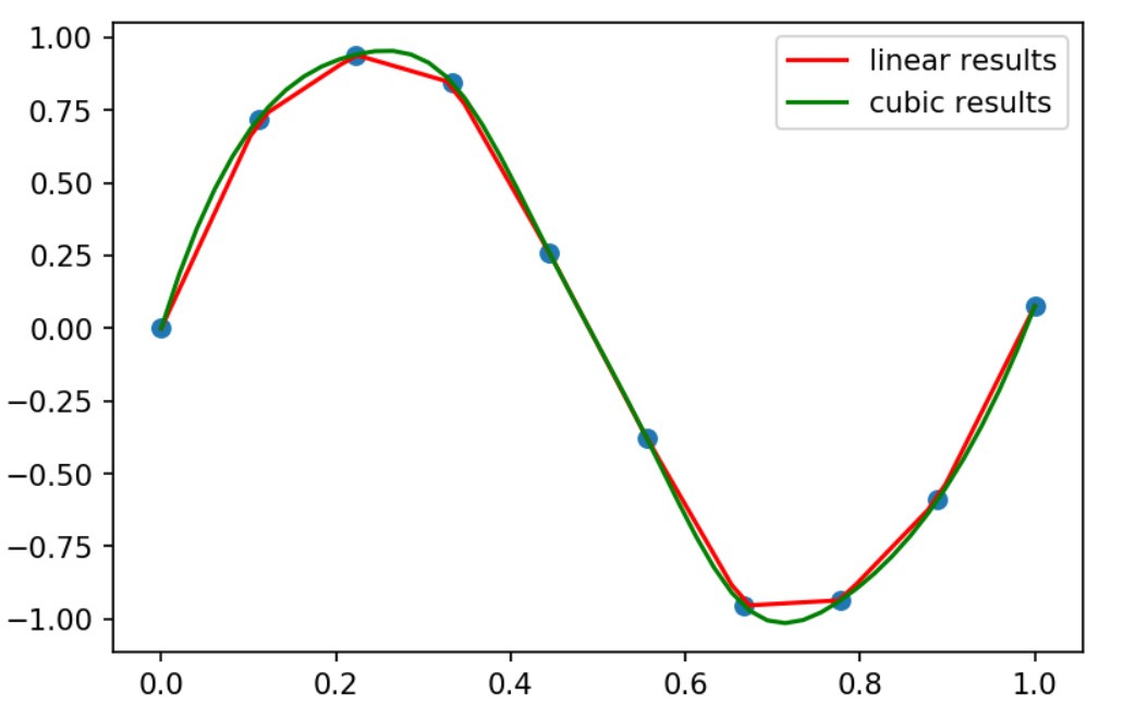
As you may note we are trying out the linear and cubic interpolation and using the scipy.interpolate.interp1d function.
Statistics
In here I will combine pandas data loading with scipy.stats module.
import pandas as pd
import io
text=u'''
"";"Gender";"FSIQ";"VIQ";"PIQ";"Weight";"Height";"MRI_Count"
"1";"Female";133;132;124;"118";"64.5";816932
"2";"Male";140;150;124;".";"72.5";1001121
"3";"Male";139;123;150;"143";"73.3";1038437
"4";"Male";133;129;128;"172";"68.8";965353
"5";"Female";137;132;134;"147";"65.0";951545
'''

pd.read_csv
df=pd.read_csv(io.StringIO(text),
               sep=r';',
               na_values=".",
               header='infer', #by default
               engine='python',
               encoding = "iso-8859-1")
df
Output:
	 0 	Gender 	FSIQ 	VIQ 	PIQ 	Weight 	Height 	MRI_Count
0 	1 	Female 	133 	132 	124 	118.0 	64.5 	816932
1 	2 	Male 	140 	150 	124 	NaN 	72.5 	1001121
2 	3 	Male 	139 	123 	150 	143.0 	73.3 	1038437
3 	4 	Male 	133 	129 	128 	172.0 	68.8 	965353
4 	5 	Female 	137 	132 	134 	147.0 	65.0 	951545
After data load, here is how to create Student’s t-test or the simplest statistical test (part of hypothesis testing).
from pandas import plotting
#plotting.scatter_matrix(df[['Weight', 'Height', 'MRI_Count']])
from scipy import stats
r1 = stats.ttest_1samp(df['VIQ'], 0)
female_viq = df[df['Gender'] == 'Female']['VIQ']
male_viq = df[df['Gender'] == 'Male']['VIQ']
r2 = stats.ttest_ind(female_viq, male_viq)
# testing the value of a population mean
print(r1)
# testing for difference across populations
print(r2)
Output:
Ttest_1sampResult(statistic=29.53444067255562, pvalue=7.825719971719742e-06)
Ttest_indResult(statistic=-0.18926408936295352, pvalue=0.8619667118907584)
| Column | Description |
|---|---|
| Gender | Male or Female |
| FSIQ | Full Scale IQ scores based on the four Wechsler (1981) subtests |
| VIQ | Verbal IQ scores based on the four Wechsler (1981) subtests |
| PIQ | Performance IQ scores based on the four Wechsler (1981) subtests |
| Weight | body weight in pounds |
| Height | height in inches |
| MRI_Count | total pixel Count from the 18 MRI scans |
Scipy.stats vs. Statsmodels
Although statsmodels is not part of scipy.stats they work great in tandem.some very important functions worth to mention in here.
Statsmodels has scipy.stats as a dependency.
Scipy.stats has all of the probability distributions and some statistical tests. It’s more like library code in the vein of numpy and scipy.
Statsmodels on the other hand provides statistical models with a formula framework similar to R and it works with pandas out of the box.
Statsmodels has statistical tests, plotting, and plenty of helper functions.
Example:
import numpy as np
# feature
x = np.linspace(-10, 10, 20)
np.random.seed(13)
# target
y = -5 + 3*x + 4 * np.random.normal(size=x.shape)
df = pd.DataFrame({'x': x, 'y': y})
from statsmodels.formula.api import ols
model = ols("y ~ x", df).fit()
print(model.summary())
Output:
OLS Regression Results
==============================================================================
Dep. Variable:                      y   R-squared:                       0.944
Model:                            OLS   Adj. R-squared:                  0.941
Method:                 Least Squares   F-statistic:                     302.5
Date:                Sun, 26 Apr 2020   Prob (F-statistic):           1.06e-12
Time:                        21:40:26   Log-Likelihood:                -57.988
No. Observations:                  20   AIC:                             120.0
Df Residuals:                      18   BIC:                             122.0
Df Model:                           1
Covariance Type:            nonrobust
==============================================================================
                 coef    std err          t      P>|t|      [0.025      0.975]
------------------------------------------------------------------------------
Intercept     -5.5335      1.036     -5.342      0.000      -7.710      -3.357
x              2.9684      0.171     17.393      0.000       2.610       3.327
==============================================================================
Omnibus:                        0.100   Durbin-Watson:                   2.956
Prob(Omnibus):                  0.951   Jarque-Bera (JB):                0.322
Skew:                          -0.058   Prob(JB):                        0.851
Kurtosis:                       2.390   Cond. No.                         6.07
==============================================================================

Warnings:
[1] Standard Errors assume that the covariance matrix of the errors is correctly specified.
…
tags: scipy & category: python