Scikit-learn (sklearn) examples

Table of contents:
- What can we do with Scikit-learn?
- Installation
- Dependencies
- Mission as a reference
- Splitting the train and test set
- Datasets
- Estimators
- Pipeline
- Metrics
- Models
- Decision Trees
- Ensembles
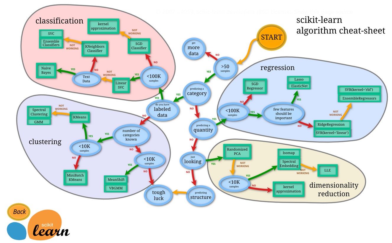
What can we do with Scikit-learn?
Scikit-learn (also known as sklearn) is the first association for “Machine Learning in Python”. This package helps solving and analyzing different classification, regression, clustering problems. It includes SVM, and interesting subparts like decision trees, random forests, gradient boosting, k-means, KNN and other algorithms. It uses NumPy and SciPy as core dependencies.
Installation
From the official website you will find that the correct way to install is:
pip install -U scikit-learn
and the correct way to import is:
import sklearn
The scikit-learn and sklearn are synonyms.
Dependencies
When I executed:
pip show scikit-learn
I got the following feedback:
Name: scikit-learn
Version: 0.22.2.post1
Summary: A set of python modules for machine learning and data mining
Home-page: http://scikit-learn.org
Author: None
Author-email: None
License: new BSD
Location: /usr/local/lib/python3.6/dist-packages
Requires: numpy, scipy, joblib
Required-by: yellowbrick, umap-learn, textgenrnn, sklearn, sklearn-pandas, mlxtend, lucid, lightgbm, librosa, imbalanced-learn, fancyimpute
You can also check:
sklearn.show_versions()
Output I got:
System:
    python: 3.6.9 (default, Nov  7 2019, 10:44:02)  [GCC 8.3.0]
executable: /usr/bin/python3
   machine: Linux-4.19.104+-x86_64-with-Ubuntu-18.04-bionic

Python dependencies:
       pip: 19.3.1
setuptools: 46.1.3
   sklearn: 0.22.2.post1
     numpy: 1.18.3
     scipy: 1.4.1
    Cython: 0.29.16
    pandas: 1.0.3
matplotlib: 3.2.1
    joblib: 0.14.1

Built with OpenMP: True
Mission as a reference
Scikit-learn mission is to provide simple and efficient solutions for some machine learning problems that are nice documented and easy to use.
You may consider the scikit-learn as a reference of machine learning models, estimators, and terms.
For instance, you can split train and test set in PyTorch or TensorFlow, but this can be done with sklearn.model_selection > train_test_split.
Splitting the train and test set
In here we will have the typical example with n samples, f features with single target y.
Example:
import numpy as np
from sklearn.model_selection import train_test_split
np.random.seed(13)
n=100 # number of samples
f=10 # number of features
X,y = np.random.rand(f*n).reshape((n,f)), np.random.rand(n)
# X,y
X_train, X_test, y_train, y_test = train_test_split(X, y, test_size=0.33, random_state=13)
print(X_train.shape, y_train.shape)
print(X_test.shape, y_test.shape)
Output:
(67, 10) (67,)
(33, 10) (33,)
Datasets
Originally you can load predefined dataset.
Example wine dataset:
from sklearn.datasets import load_wine
data = load_wine()
data.target[[10, 80, 140]]

list(data.target_names)
Output:
['class_0', 'class_1', 'class_2']
Example Boston dataset 1:
from sklearn.datasets import load_boston
X,y = load_boston(return_X_y=True)
X,y
In here you will get X features and y target.
Example Boston dataset 2:
from sklearn.datasets import load_boston
X = load_boston(return_X_y=False)
X['data'],X['feature_names'], X['DESCR']
In here you will get feature names and description.
There is also a list of generator datasets:
Example:
from sklearn.datasets import make_classification
X, y = make_classification(n_samples=10, n_features=4,n_informative=2, n_redundant=0, random_state=0, shuffle=False)
X,y
Output:
(array([[-2.24080141,  0.50054121, -0.34791215,  0.15634897],
        [-1.60020786, -0.51203824,  1.23029068,  1.20237985],
        [-2.3748206 ,  0.82768797, -0.38732682, -0.30230275],
        [-1.43411205,  1.50037656, -1.04855297, -1.42001794],
        [-0.98740462,  0.99958558, -1.70627019,  1.9507754 ],
        [-1.19536732,  1.27804656, -0.50965218, -0.4380743 ],
        [ 0.29484027, -0.79249401, -1.25279536,  0.77749036],
        [ 0.6476239 , -0.81753611, -1.61389785, -0.21274028],
        [ 2.38363567,  1.56914464, -0.89546656,  0.3869025 ],
        [ 1.51783379,  1.22140561, -0.51080514, -1.18063218]]),
 array([0, 0, 0, 1, 1, 1, 0, 0, 1, 1]))
Estimators
Estimator is scikit-learn terminology for the model. An estimator is an object that learns from data using the fit method. It can be either classification, regression or clustering type of the process or even a transform operation on data. (extracts some columns from the data).
Special case of estimator is called transofrm estimator or transformer if it supports either transform or fit_transform methods.
An estimator may take parameters. The base class for all the estimators is BaseEstimator.
An estimator which takes another estimator as a parameter is called meta-estimator.
One such meta-estimator is a pipeline.Pipeline.
Pipeline
To combine multiple estimators into one use a pipeline. The Pipeline is a list of key-value pairs.
For example:
estimators = [('reduce_dim', PCA()), ('clf', SVC())]
pipe = Pipeline(estimators)
With the pipeline you modify just the features X or the data. The target y should not be modified with pipeline technique.
For example feature selection, normalization and classification may be in a pipeline.
All estimators in a pipeline, except the last one, must have a transform method (transformers).
Check last estimator type with his _estimator_type attribute of type string.
pipe[-1]._estimator_type
Transform estimators do not have _estimator_type attribute.
make_pipeline is a shortcut to create pipeline with auto keys. It fills the names automatically.
Example:
from sklearn.pipeline import make_pipeline
from sklearn.naive_bayes import MultinomialNB
from sklearn.preprocessing import Binarizer
make_pipeline(Binarizer(), MultinomialNB())
p
Output:
Pipeline(memory=None,
         steps=[('binarizer', Binarizer(copy=True, threshold=0.0)),
                ('multinomialnb',
                 MultinomialNB(alpha=1.0, class_prior=None, fit_prior=True))],
         verbose=False)
you index into estomator with
p[0]
Output:
Binarizer(copy=True, threshold=0.0)
Metrics
There are following metrics:
- Classification metrics
- Regression metrics
- Multilabel ranking metrics
- Clustering metrics
- Biclustering metrics
- Pairwise metrics
In here we briefly cover the common examples on classification and regression metrics.
Classification metrics
f1_score
F1 is an example from classification metrics. It considers both the precision p and the recall r. It works for binary classification and multiclass/multilabel targets.
Calculation:
f1 = 2pr/(p+r)
Example:
from sklearn.metrics import f1_score
y_true = [0, 1, 2, 0, 1, 2]
y_pred = [0, 2, 1, 0, 0, 1]
ma = f1_score(y_true, y_pred, average='macro')
mi = f1_score(y_true, y_pred, average='micro')
we = f1_score(y_true, y_pred, average='weighted')
no = f1_score(y_true, y_pred, average=None)
ma,mi,we,no
Output:
(0.26666666666666666,
 0.3333333333333333,
 0.26666666666666666,
 array([0.8, 0. , 0. ]))
The parameter average is binary by default. The other averages are:
- micro
- macro
- weighted
- samples and
- None
accuracy_score
Example:
from sklearn.metrics import accuracy_score
y_pred = [0, 2, 1, 3] # prediction
y_true = [0, 1, 2, 3] # true
accuracy_score(y_true, y_pred),
accuracy_score(y_true, y_pred, normalize=False)
Output:
0.5
2
Regression metrics
mean_absolute_error
Mean absolute error regression loss
\[\text{MAE}(y, \hat{y}) = \frac{1}{n_{\text{samples}}} \sum_{i=0}^{n_{\text{samples}}-1} \left| y_i - \hat{y}_i \right|\]Example:
from sklearn.metrics import mean_absolute_error
y_true = [3, -0.5, 2, 7]
y_pred = [2.5, -0.4, 2, 8]
r1 = mean_absolute_error(y_true, y_pred)
y_true = [[0.5, 1], [-1, 1], [7, -6]]
y_pred = [[0, 2], [-1, 2], [8, -5]]
r2 = mean_absolute_error(y_true, y_pred)
r3 = mean_absolute_error(y_true, y_pred, multioutput='raw_values')
r4 = mean_absolute_error(y_true, y_pred, multioutput=[0.3, 0.7])
r1,r2,r3,r4
Output:
(0.4, 0.75, array([0.5, 1. ]), 0.85)
mean_squared_error
\[\text{MSE}(y, \hat{y}) = \frac{1}{n_\text{samples}} \sum_{i=0}^{n_\text{samples} - 1} (y_i - \hat{y}_i)^2\]Example:
from sklearn.metrics import mean_squared_error
y_true = [3, -0.5, 2, 7]
y_pred = [2.5, 0.0, 2, 8]
r1 = mean_squared_error(y_true, y_pred)
y_true = [[0.5, 1], [-1, 1], [7, -6]]
y_pred = [[0, 2], [-1, 2], [8, -5]]
r2 = mean_squared_error(y_true, y_pred)
r1,r2
Output:
(0.375, 0.7083333333333334)
mean_squared_log_error
The mean_squared_log_error function computes a risk metric corresponding to the expected value of the squared logarithmic (quadratic) error or loss.
\[\text{MSLE}(y, \hat{y}) = \frac{1}{n_\text{samples}} \sum_{i=0}^{n_\text{samples} - 1} (\log_e (1 + y_i) - \log_e (1 + \hat{y}_i) )^2\]Example:
from sklearn.metrics import mean_squared_log_error
y_true = [3, 5, 2.5, 7]
y_pred = [2.5, 5, 4, 8]
r1 = mean_squared_log_error(y_true, y_pred)
y_true = [[0.5, 1], [1, 2], [7, 6]]
y_pred = [[0.5, 2], [1, 2.5], [8, 8]]
r2 = mean_squared_log_error(y_true, y_pred)
r1,r2
Output:
(0.039, 0.044)
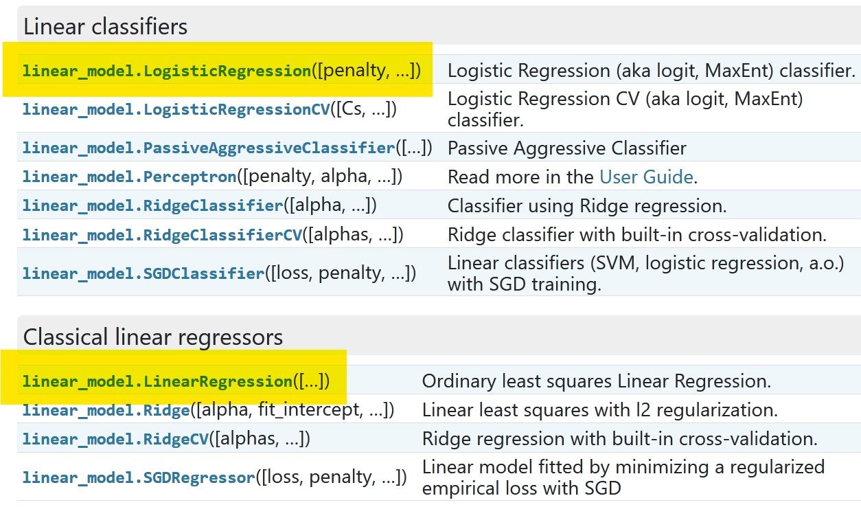
Models
Example models that are often used are: LogisticRegression, that is a classifier model itself, and LinearRegression that is a regression model.
Example:
from sklearn.datasets import load_iris
from sklearn.linear_model import LogisticRegression
X,y = load_iris(return_X_y=True)
clf = LogisticRegression(random_state=0, solver='liblinear', multi_class='auto').fit(X, y)
r1 = clf.predict(X[:2, :])
r2 = clf.predict_proba(X[:2, :])
r3 = clf.score(X, y)
r1,r2,r3
Output:
(array([0, 0]), array([[8.78030305e-01, 1.21958900e-01, 1.07949250e-05],
        [7.97058292e-01, 2.02911413e-01, 3.02949242e-05]]), 0.96)
Example:
import numpy as np
from sklearn.linear_model import LinearRegression
X = np.array([[1, 1], [1, 2], [2, 2], [2, 3]])
# y = 1 * x_0 + 2 * x_1 + 3
y = np.dot(X, np.array([1, 2])) + 3
reg = LinearRegression().fit(X, y)
r1 = reg.score(X, y)
r2 = reg.coef_
r3 = reg.intercept_
r4 = reg.predict(np.array([[3, 5]]))
r1,r2,r3,r4
Output:
(1.0, array([1., 2.]), 3.0000000000000018, array([16.]))
Cross Validation
Once we have the prediction model we need to evaluate model precision on unseen data. While training, we don’t have unseen data in advance and is a common practice to hold out part of the available data known as a test set.
This can be done with cross validation applied together with the prediction model.
Here are some common imports for cross validation:
from sklearn.model_selection import cross_val_score
from sklearn.model_selection import cross_val_prediction
from sklearn.model_selection import cross_validate
Example:
from sklearn import datasets, linear_model
from sklearn.model_selection import cross_val_score
diabetes = datasets.load_diabetes()
X = diabetes.data[:150]
y = diabetes.target[:150]
lasso = linear_model.Lasso()
print(cross_val_score(lasso, X, y, cv=3))
Output:
[0.33150734 0.08022311 0.03531764]
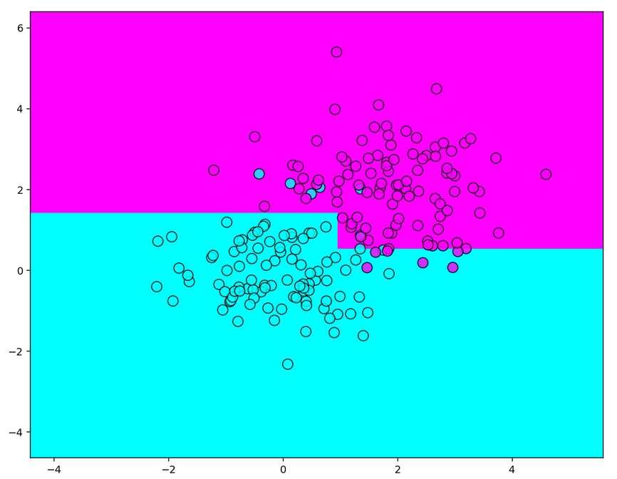
Decision Trees
You use decision trees forms often:
from sklearn.tree import DecisionTreeRegressor
from sklearn.tree import DecisionTreeClassifier
Example:
import numpy as np
from matplotlib import pyplot as plt

np.random.seed(13)
train_data = np.random.normal(size=(100, 2))
train_labels = np.zeros(100)

# adding second class
train_data = np.r_[train_data, np.random.normal(size=(100, 2), loc=2)]
train_labels = np.r_[train_labels, np.ones(100)]

from sklearn.tree import DecisionTreeClassifier

r = 150 # resolution
x = np.linspace(2*train_data[:, 0].min(), train_data[:, 0].max()+1, num=r)
y = np.linspace(2*train_data[:, 1].min(), train_data[:, 1].max()+1, num=r)
xx,yy = np.meshgrid(x, y)

clf_tree = DecisionTreeClassifier(criterion='entropy', max_depth=2) # gini

# training = fitting
clf_tree.fit(train_data, train_labels)

# predicting (with the resolution shape of rXr)
predicted = clf_tree.predict(np.c_[xx.ravel(), yy.ravel()]).reshape(xx.shape)
plt.figure(figsize=(10,8), dpi=140)
plt.pcolormesh(xx, yy, predicted, cmap='cool')
plt.scatter(train_data[:, 0], train_data[:, 1], c=train_labels, s=100, alpha=0.8,
            edgecolors='black', cmap='cool')
Output:
Ensembles
Random Forests
The following RF are frequent in use:
from sklearn.ensemble import RandomForestClassifier
from sklearn.ensemble import RandomForestRegressor
Example:
from sklearn.ensemble import RandomForestClassifier
from sklearn.datasets import make_classification

X, y = make_classification(n_samples=1000, n_features=4, n_informative=2, n_redundant=0, random_state=0, shuffle=False)
clf = RandomForestClassifier(max_depth=2, random_state=0, n_estimators=20)
clf.fit(X, y)
print(clf.feature_importances_)
print(clf.predict([[0, 0, 0, 0]]))
Output:
[0.15733456 0.79341435 0.0222356  0.02701549]
[1]
AdaBoost
The core principle of AdaBoost is to fit a sequence of weak learners. Weak learners are models that are slightly better than random guessing (typically small decision trees).
The predictions from weak learners are combined to a weighted sum to produce the better prediction.
Often in use:
from sklearn.ensemble import AdaBoostClassifier
from sklearn.ensemble import AdaBoostRegressor
Example:
from sklearn.model_selection import cross_val_score
from sklearn.datasets import load_iris
from sklearn.ensemble import AdaBoostClassifier

X, y = load_iris(return_X_y=True)
clf = AdaBoostClassifier(n_estimators=100)
scores = cross_val_score(clf, X, y, cv=5)
scores.mean()
Output:
0.9
GradientBoosting
Can be used for both regression and classification problems in a variety of areas including Web search ranking.
This is an iterative technique which adjusts the weight of an observation based on the previous predictions.
Often in use:
from sklearn.ensemble import GradientBoostingClassifier
from sklearn.ensemble import GradientBoostingRegressor
Example:
from sklearn.datasets import make_hastie_10_2
from sklearn.ensemble import GradientBoostingClassifier

X, y = make_hastie_10_2(random_state=0)
X_train, X_test = X[:2000], X[2000:]
y_train, y_test = y[:2000], y[2000:]

clf = GradientBoostingClassifier(n_estimators=100, learning_rate=1.0,
    max_depth=1, random_state=0).fit(X_train, y_train)
clf.score(X_test, y_test)
Output:
0.913
Bagging
Bagging from bootstrap aggregating.
Bagging is technique to generate the additional data from the original dataset. This should decrease the variance in the precision.
Math equivalent would be combinations with repetitions.
It is usually applied to decision trees, but it can be used with any type of method.
Often in use:
from sklearn.ensemble import BaggingClassifier
from sklearn.ensemble import BaggingRegressor
Example:
from sklearn.svm import SVC
from sklearn.ensemble import BaggingClassifier
from sklearn.datasets import make_classification
X, y = make_classification(n_samples=100, n_features=4,
                           n_informative=2, n_redundant=0,
                           random_state=0, shuffle=False)
clf = BaggingClassifier(base_estimator=SVC(),
                        n_estimators=10, random_state=0).fit(X, y)
clf.predict([[0, 0, 0, 0]])
Output:
array([1])
…
tags: examples - data analysis - machine learning & category: python