PyTorch | Automatic Differentiation

Table of Contents:
- What is PyTorch AD ?
- Create backward computational graph using torchviz
- Detach from AD
- Bonus define deep learning
What is PyTorch AD ?
Automatic Differentiation (AD) is a technique to calculate the derivative of function $f(x_1, \cdots, x_n)$ at some point.
What PyTorch AD is not ?
AD is not symbolic math approach to calculate the derivate. Symbolic math approach would be to use derivation rules. For example, if you have $f(x) = {1\over x}$ then $f’(x) = -{1 \over x^2}$.
AD is also not numeric procedure to calculate the derivate. The numerical procedure to calculate the derivative of tanh function at point $x=1$ would be:
def tanh(x):
  y=np.exp(-x)
  return (1.0-y)/(1.0+y)

s=0.00001 # some small number
x=1.0
d=(tanh(x+s)-tanh(x))/s
print(d)
Output:
0.39322295790622513
How reverse mode AD works?
PyTorch uses reverse mode AD. AD forward mode exists, but it is computationally more expensive.
Reverse mode AD works the following way.
First the forward pass is being executed. In the forward pass PyTorch creates the computational graph dynamically and calculates the intermediate variables based on inputs.
The computational graph being calculated is like a tree. Inputs are tree leaves and each node in the graph corresponds to some operation (such as +), or to some function (such as sin).
The output function is the root of the tree. Once we create the computational tree in the forward pass, together with the intermediate gradients, we then may get the gradients from the root to any of the leaves.
We say: we compute the gradients of a function with respect to the input variable $x$.
This pass when we compute the gradients is known as the backward pass and corresponds to PyTorch grad funciton.
PyTorch grad function is very cheap. It just traverses the computational graph and creates the sum of the intermediate gradient products to calculate the final gradient. The math behind calculating gradient is called the chain rule.
Note: There is one tool similar to Pytorch called Chainer just because of this chain rule principle.
Example:
To get a clue how PyTorch AD works the next code example we will create the computational graph for the function:
\[f(x_1, x_2) = \frac{ 1+sin(x_2)}{x_2+e^{x_1}} + x_1x_2\]We will calculate the gradient of a function $f(x_1, x_2)$ with respect to $x_2$.
import math
class ADNumber:

    def __init__(self,val, name=""):
        self.name=name
        self._val=val
        self._children=[]

    def __truediv__(self,other):
        new = ADNumber(self._val / other._val, name=f"{self.name}/{other.name}")
        self._children.append((1.0/other._val,new))
        other._children.append((-self._val/other._val**2,new)) # first derivation of 1/x is -1/x^2
        return new

    def __mul__(self,other):
        new = ADNumber(self._val*other._val, name=f"{self.name}*{other.name}")
        self._children.append((other._val,new))
        other._children.append((self._val,new))
        return new

    def __add__(self,other):
        if isinstance(other, (int, float)):
            other = ADNumber(other, str(other))
        new = ADNumber(self._val+other._val, name=f"{self.name}+{other.name}")
        self._children.append((1.0,new))
        other._children.append((1.0,new))
        return new

    def __sub__(self,other):
        new = ADNumber(self._val-other._val, name=f"{self.name}-{other.name}")
        self._children.append((1.0,new))
        other._children.append((-1.0,new))
        return new


    @staticmethod
    def exp(self):
        new = ADNumber(math.exp(self._val), name=f"exp({self.name})")
        self._children.append((self._val,new))
        return new

    @staticmethod
    def sin(self):
        new = ADNumber(math.sin(self._val), name=f"sin({self.name})")
        self._children.append((math.cos(self._val),new)) # first derivation is cos
        return new

    def grad(self,other):
        if self==other:
            return 1.0
        else:
            result=0.0
            for child in other._children:
                result+=child[0]*self.grad(child[1])
            return result

A = ADNumber # shortcuts
sin = A.sin
exp = A.exp

def print_child(f, wrt): # with respect to
    for e in f._children:
        print("child:", wrt, "->" , e[1].name, "grad: ", e[0])
        print_child(e[1], e[1].name)


x1 = A(1.5, name="x1")
x2 = A(0.5, name="x2")
f=(sin(x2)+1)/(x2+exp(x1))+x1*x2

print_childs(x2,"x2")
print("\ncalculated gradient for the function f with respect to x2:", f.grad(x2))
Out:
child: x2 -> sin(x2) grad:  0.8775825618903728
child: sin(x2) -> sin(x2)+1 grad:  1.0
child: sin(x2)+1 -> sin(x2)+1/x2+exp(x1) grad:  0.20073512936690338
child: sin(x2)+1/x2+exp(x1) -> sin(x2)+1/x2+exp(x1)+x1*x2 grad:  1.0
child: x2 -> x2+exp(x1) grad:  1.0
child: x2+exp(x1) -> sin(x2)+1/x2+exp(x1) grad:  -0.05961284871202578
child: sin(x2)+1/x2+exp(x1) -> sin(x2)+1/x2+exp(x1)+x1*x2 grad:  1.0
child: x2 -> x1*x2 grad:  1.5
child: x1*x2 -> sin(x2)+1/x2+exp(x1)+x1*x2 grad:  1.0

calculated gradient for the function f with respect to x2: 1.6165488003791766
Check:
1.5 + (0.8775825618903728 * 1.0 * 0.20073512936690338) + (-0.05961284871202578 *1.0)
Out:
1.6165488003791768
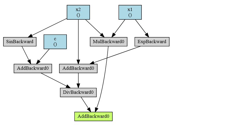
The next image shows the computational graph for the example function:
\[f(x_1, x_2) = \frac{ 1+sin(x_2)}{x_2+e^{x_1}} + x_1x_2\]where
$x_1=1.5, x_2=0.5$

Each node in the tree graph is either a leaf node (green) or the root node (brown) or something in between.
From the input x2 in forward pass we identify three paths leading to the root. The arrows in dark red, red and orange denote these paths. We can ignore black arrows for now.
To compute the final gradient for our function f with respect to the x2 we need to multiply the gradient values along the paths and finally to sum them up.
The calculus is as follows:
1.5 + (0.8775825618903728 * 1.0 * 0.20073512936690338) + (-0.05961284871202578 *1.0)
# 1.6165488003791768
This is exactly what our function grad will do if we print f.grad(x2) the result will be 1.6165488003791766.
Let’s show the numerical procedure will provide the same result.
import math
def f(x1, x2):
    return (math.sin(x2)+1)/(x2+math.exp(x1))+x1*x2

e=0.0001 # some small e
x1 = 1.5
x2 = 0.5

grad = (f(x1, x2+e)-f(x1, x2))/e
print(grad) # 1.6165416488078677
Create backward computational graph using torchviz
# !pip install torchviz
from torchviz import make_dot

# Create tensors
x1 = torch.tensor(1.5, requires_grad=True)
x2 = torch.tensor(0.5, requires_grad=True)
c = torch.tensor(1., requires_grad=True)

# Build a computational graph
y=(torch.sin(x2)+c)/(x2+torch.exp(x1))+x1*x2
y.backward() # compute gradients

print(x1.grad)
print(x2.grad)
print(c.grad)

params = {'x1': x1, 'x2':x2, 'c': c}
param_map = {id(v): k for k, v in params.items()}
param_map

make_dot(y, {'x1': x1, 'x2':x2, 'c': c})
Out:
tensor(0.2328)
tensor(1.6165)
tensor(0.2007)
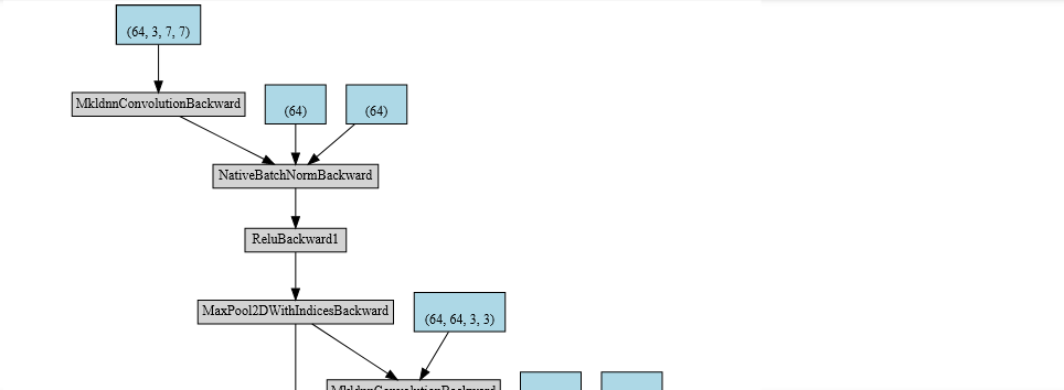
Example: Create resnet18 computational graph
import torch
import torchvision.models as models
resnet18 = models.resnet18()
x = torch.zeros(1, 3, 224, 224, dtype=torch.float, requires_grad=False)
out = resnet18(x)
make_dot(out)
Example: Using hiddenlayer
import torch
import hiddenlayer as hl
import torchvision.models as models
resnet18 = models.resnet18()
x = torch.zeros(1, 3, 224, 224, dtype=torch.float, requires_grad=False)

transforms = [ hl.transforms.Prune('Constant') ] # removes Constant nodes from graph.
# resnet18 from torchvision and and x is the input 4D tensor
graph = hl.build_graph(resnet18, x, transforms=transforms)
graph.theme = hl.graph.THEMES['blue'].copy()
# graph.save('rnn_hiddenlayer', format='png')
graph
 Save and zoom to check the details
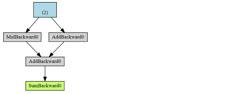
Detach from AD
Here is one computational graph.
from torchviz import make_dot
x=torch.ones(2, requires_grad=True)
y=2*x
z=3+x
r=(y+z).sum()
make_dot(r)
It is possible to detach() the tensor from the AD computational graph.
from torchviz import make_dot
x=torch.ones(2, requires_grad=True)
y=2*x
z=3+x.detach()
r=(y+z).sum()
make_dot(r)
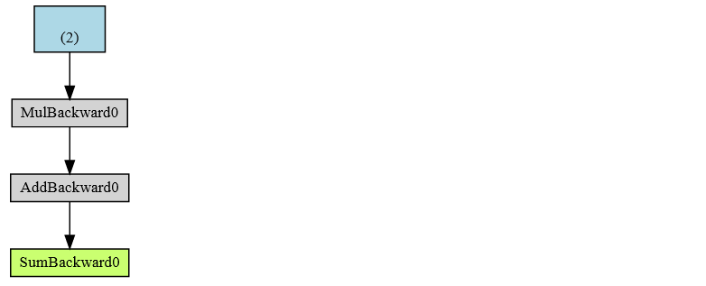
x.detach()is the same asx.data.
from torchviz import make_dot
x=torch.ones(2, requires_grad=True)
y=2*x
z=3+x.data
r=(y+z).sum()
make_dot(r)
You can use the with torch.no_grad() class (context manager). Whatever is created inside that block, will end as requires_grad=False. The next example will show just that. Tensor x that requires_grad=True will create tensor y, but that tensor will have requires_grad=False.
x=torch.tensor(2., requires_grad=True)
print(x)
with torch.no_grad():
    y = x * 2
print(y, y.requires_grad)
Out:
tensor(2., requires_grad=True)
tensor(4.) False
For more details refer to help(torch.no_grad).
Bonus define deep learning
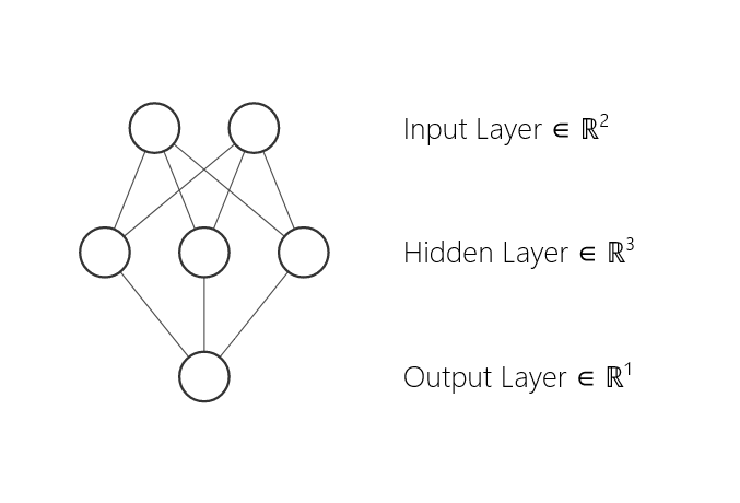
In essence, for the deep learning you need to have deep models. By definition, shallow models have just one hidden layer:
model = torch.nn.Sequential(
          torch.nn.Linear(D_in, H),
          torch.nn.Linear(H, D_out),
        )
Deep models have 2 or more hidden layers.
model = torch.nn.Sequential(
          torch.nn.Linear(D_in, H1),
          torch.nn.Linear(H1, H2),
          torch.nn.Linear(H2, D_out),
        )
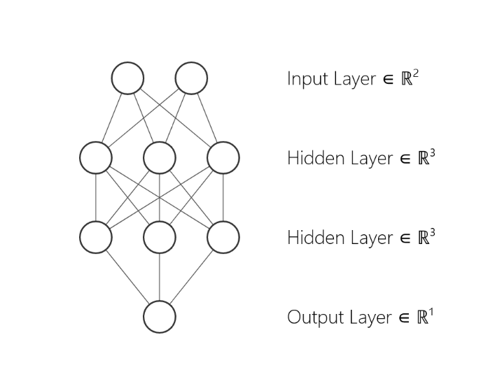
In other words, to do some deep learning you need to have at least three linear layers. The dimension H is called the hidden dimension. Instead of nn.Linear layers you may use convolution layers.
…
tags: ad - pytorch automatic differentiation - pytorch ad - automatic differentiation - computational graph - backward computational graph - reverse mode ad - derivation rule & category: pytorch