PyTorch | Train and Save the Model

PyTorch training steps

In here, we have a PyTorch training model when we use loss function looks like this:

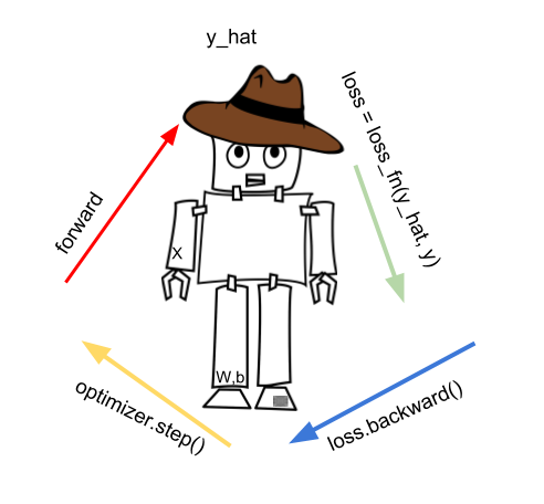
There are characteristic phases:

• forward pass
• calculating the loss
• backward pass
• updating the parameters
• zero the gradients
• pytorch epoch

As this is the foundation, optionally we may tweak the learning rate using the learning rate scheduler. Learning rate is a hyperparameter.

Most notable is the forward pass where we step into the model and predict the y_hat. We can write this as a function:

def fit():    
    y_hat = model(X) # forward pass
    loss = loss_fun(y_hat, y)    
    loss.backward()
    opt.step()
    opt.zero_grad()

We compute predicted y_hat by passing X to the model. y_hat is also known as prediction. Then we take into account the loss function loss_fn to get the loss. We first zero the gradients as these are accumulators, then we do the back propagation, and optimization step. Optimization step will update our parameters, weights and biases.

But the data is huge we cannot get the loss for all the data at once, and we divide out X into batches. This way we have the following fit function:

def fit():
    for epoch in range(epochs):
        for xb, yb in train.dl:
            y_hat = model(xb)# one batch
            loss = loss_fun(y_hat, yb)            
            loss.backward()
            opt.step()
            opt.zero_grad()

In here we took into account the batches xb and yb.

Our model may be for instance the simplest deep learning model:

model = torch.nn.Sequential(
          torch.nn.Linear(D_in, H),
          torch.nn.Linear(H, D_out),
        )

The model can be either:

torch.nn.Sequential
torch.nn.Functional

What we get from the model forward phase is the y_hat, or the prediction.

We use that prediction to create the loss, using the loss_fn (the loss function)

loss = loss_fn(y_hat, y)

Sum of all loss values is the error, but we may also say total loss. One of the most common used loss function is the Euclid distance loss:

loss_fn = torch.nn.MSELoss()

Once we calculate the loss we call loss.backward(). The loss.backward() will calculate the gradients automatically. Gradients are needed in the next phase, when we use the optimizer.step() function to improve our model parameters.

We can get all our model parameters via: model.parameters() method. Once we update model parameters, we repeat the forward phase again.

In our example we used the torch.nn.Linear() layer, to transformation the input in linear way (matrix multiplication). A non-linear transformation follows the Linear layer since this is know neural networks can best learn.

Note that each PyTorch forward phase creates the calculation graph; thanks to that graph we compute the gradients.

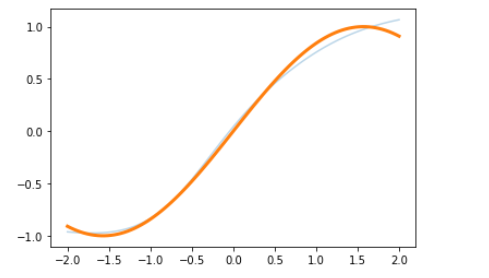
Example: Training

We first create the model with two linear layers, then use SGD optimizer and run 200 iteration steps.

Simplified: In each step we calculate the loss, run the backward() on that loss and zero the gradients.

import torch 

model=torch.nn.Sequential(
    torch.nn.Linear(1,10),
    torch.nn.Tanh(),
    torch.nn.Linear(10,1))

opt=torch.optim.SGD(model.parameters(),lr=1e-2)

for i in range(200):
    x=torch.randn(10,1)# input from dataset
    target=torch.sin(x)# target from dataset
    
    pred=model(x)
    loss=torch.nn.functional.mse_loss(pred,target,reduction='sum')
    
    opt.zero_grad()
    loss.backward()
    opt.step()  

To show the results of what we done:

%matplotlib inline
import matplotlib.pyplot as plt

with torch.no_grad():
    x0=torch.linspace(-2,2)
    plt.plot(x0,model(x0[:,None]).detach(),alpha=0.3)
    plt.plot(x0,torch.sin(x0),linewidth=3)
    plt.show()

Saving the model

Saving models has two typical scenarios:

• save the model for inference
• save the model for later training

PyTorch models do have two dictionaries inside so called “state dicts”:

• learnable parameters state_dict
• optimizer state_dict

Learnable parameters are the first state_dict. The PyTorch model torch.nn.Module has model.parameters() call to get learnable parameters ($W$ and $b$). These learnable parameters, once randomly set, will update over time as we learn.

The second state_dict is the optimizer state dict. You recall that the optimizer is used to improve our learnable parameters. But the optimizer state_dict is fixed.

Because state_dict objects are Python dictionaries, they can be easily saved, updated, altered, and restored, adding a great deal of modularity to PyTorch models and optimizers.

Example : Save model for inference

torch.save(model.state_dict(), 's.pt')

And to use it later call:

model.load_state_dict(torch.load('s.pt')) 
model.eval() 

Example : Save model for inference second way

This alternative saves the whole model but doesn’t save the optimizer state dict. So it is just for inference.

torch.save(model, 'm.pt')
model = torch.load('m.pt')
model.eval()

Example : Save model for later training

state = {
    'epoch': epoch,
    'lr_sched': lr_sched
    'state_dict': model.state_dict(),
    'optimizer': optimizer.state_dict()    
}
torch.save(state, 's.pt')

To use it:

state = torch.load('s.pt')
epoch = state['epoch']
lr_sched = state['lr_sched']
model.load_state_dict(state['state_dict'])
optimizer.load_state_dict(state['optimizer'])

Example: Save model for later training second way

You save the checkpoint at certain time:

state = { 
    'epoch': epoch,
    'model': model,
    'optimizer': optimizer,
    'lr_sched': lr_sched
}
torch.save(state, 's.pt')

Later use the model like this:

state = torch.load('s.pt')
epoch = state['epoch']
model = state['model']
optimizer = state['optimizer']
lr_sched = state['lr_sched']