Binomial distribution in R | Examples

The binomial distribution with parameters $n$ and $p$ is the discrete probability distribution.

You can write $B(n,p)$, where $n$ is the number of trials, and $p$ is the probability of success. For the binomial distribution, the random variable is $K$, the number of successes, and it has expected value $μ=np$ and variance $σ^2=np(1−p)$.

It can be represented with this formula:

$\mathbb P(X=x)={ }^{n} C_{x} p^{x}(1-p)^{n-x}$

Pre requisites

We can use Binomial distribution if the following prerequisites are present:

• There are two potential outcomes per trial
• The probability of success $p$ is the same across all trials
• The number of trials $n$ is fixed
• Each trial is independent

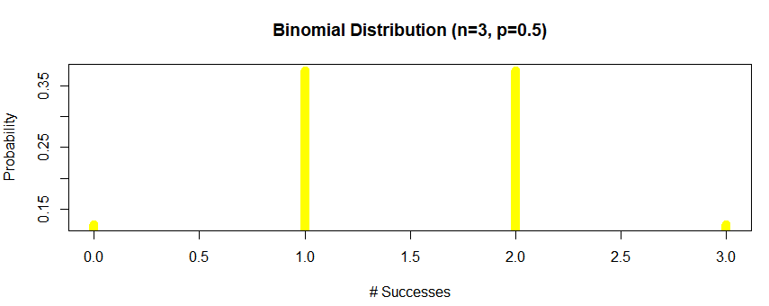
Example: We coin toss three times, what is the chance of getting two heads if the coin is fair.

Coin toss example is probably the most famous example of binomial distribution.

First we will prove that all Binomial distribution prerequisites are meat for the coin toss example. There are two potential outcomes where the probability of the success is the same $p=0.5$ we have $n=3$ trial and each trial is independent.

$\mathbb P(X=2) = {}^3C_2 p^2q^1 =\frac{3}{8}=0.375$.

We can use R code to calculate all the discrete probabilities.

dbinom(success,size=3,prob=.5)

Out:

0.125 0.375 0.375 0.125

We can plot:

success <- 0:3
plot(success,dbinom(success,size=3,prob=.5),
     type='h',
     main='Binomial Distribution (n=3, p=0.5)',
     col='yellow',
     ylab='Probability',
     xlab ='# Successes',
     lwd=10)

Same example but now $n=30$ to get a nice graph of a discrete variable.

success <- 0:50
plot(success,dbinom(success,size=30,prob=.5),
     type='h',
     main='Binomial Distribution (n=30, p=0.5)',
     col='yellow',
     ylab='Probability',
     xlab ='# Successes',
     lwd=10)

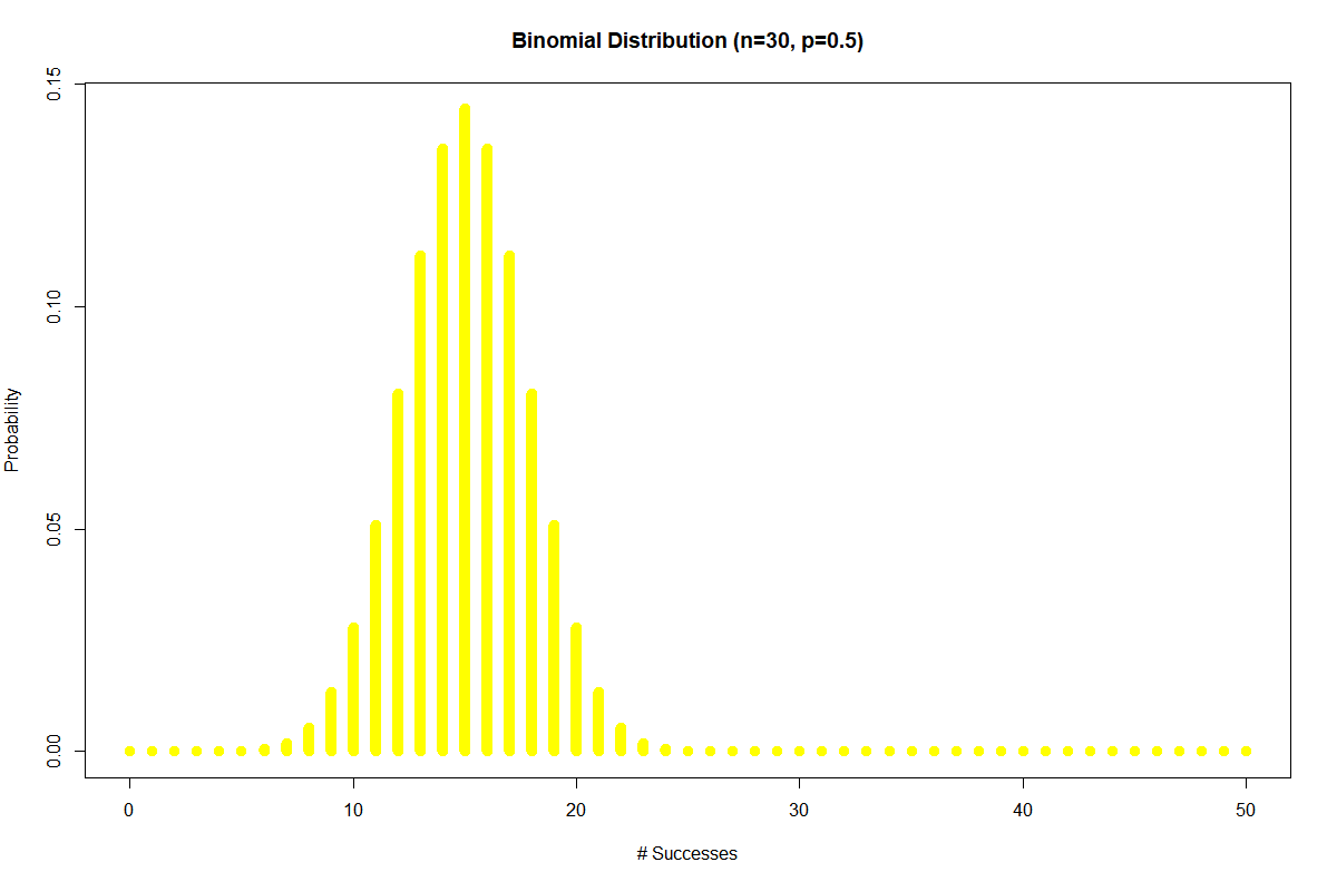
Note how the mode of the distribution is at 15.

R code for binomial distribution calculus is this:

dbinom(x, size, prob)
pbinom(x, size, prob)
qbinom(p, size, prob)
rbinom(n, size, prob)

Here dbinom is PDF, pbinom is CMF or distribution function, qbinom gives the quantile function and rbinom generates random deviations.

Example: Find $\mathbb P(X \ge 5)$ for binomial distribution with $n=20$ and $p=0.05$

Plotting the distribution first

success <- 0:20
plot(success,dbinom(success,size=20,prob=.05),
     type='h',
     main='Binomial Distribution (n=20, p=0.05)',
     ylab='Probability',
     xlab ='# Successes',
     col='yellow',
     lwd=10)

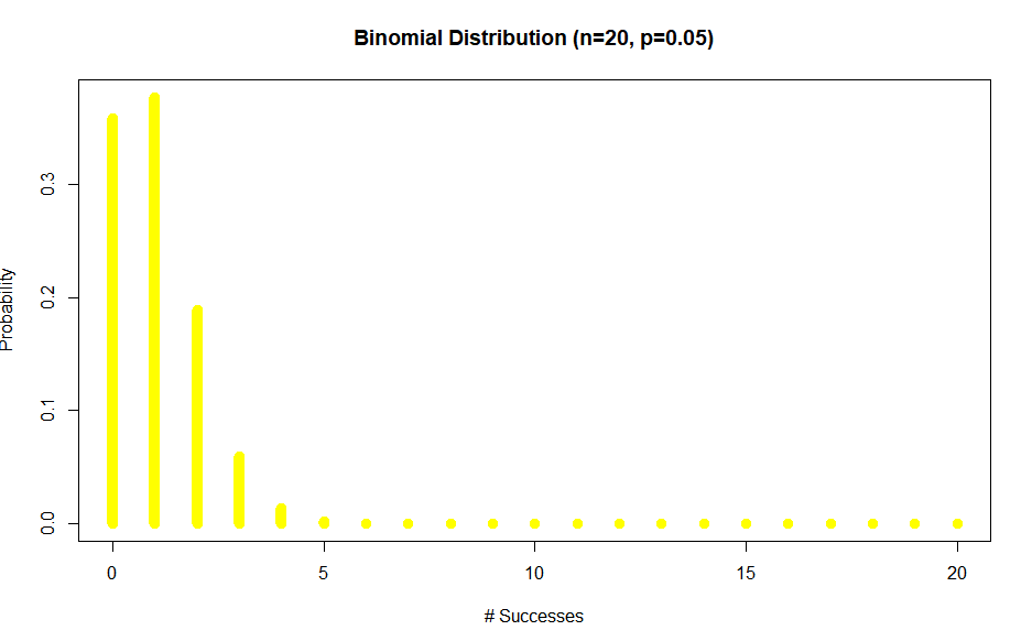
Let’s get the $\mathbb P(X \ge 5)$

1-pbinom(5,size=20,prob=0.05)

Out:

0.0003292943

Expected value and variance for binomial distribution

a) $\mathbb E\left(Y_{n}\right)=n p$

$\mathbb{E}\left(X_{i}\right)=p$ for each $i$ since independence of each trial. From the additive property of expected value:

b) $\operatorname{var}\left(Y_{n}\right)=n p(1-p)$

$\operatorname{var}\left(X_{i}\right)=p(1-p)$ for each $i$. Hence from the additive property of variance for independent variables:

Bernoulli trial

Bernoulli trial or binomial trial is a random experiment with exactly two possible outcomes:

• success
• failure

Where the probability of success is constant during the experiment.

It is named after Jacob Bernoulli from Switzerland.

Negative binomial distribution

It is very close to binomial distribution. Both distributions are based on binomial trials.

The difference is:

Random variable $Y$ is the number of trials until the $r$-th success is observed. In this case, we keep increasing the number of trials until we reach $r$ successes.

The possible values of $Y$ are $r$, $r+1$, $r+2$, … with no upper bound.

The Negative Binomial can also be defined in terms of the number of failures until the $r$-th success and this is why it is called negative binomial.

Summary

Binomial:

• formula $B(n,p)$
• fixed number of trials ($n$)
• fixed probability of success ($p$)
• number of successes is random variable $X$

Negative Binomial:

• formula $NB(r,p)$
• fixed number of successes (r)
• fixed probability of success (p)
• number of trials is random variable $Y$ until we reach the $r$-th success