Chi Squared distribution in R| Examples

Table of Contents:
- Single degree of freedom
- Two degrees of freedom
- Moments
- Goodness of fit test
- Test For Independence
- De Moivre-Laplace theorem
- Conclusion
Discovered by Robert Helmert in 1875 chi-squared distribution is one of the most frequent distributions in statistics. It can be thought of as the “square” of a Z (standard normal distribution).
Single degree of freedom
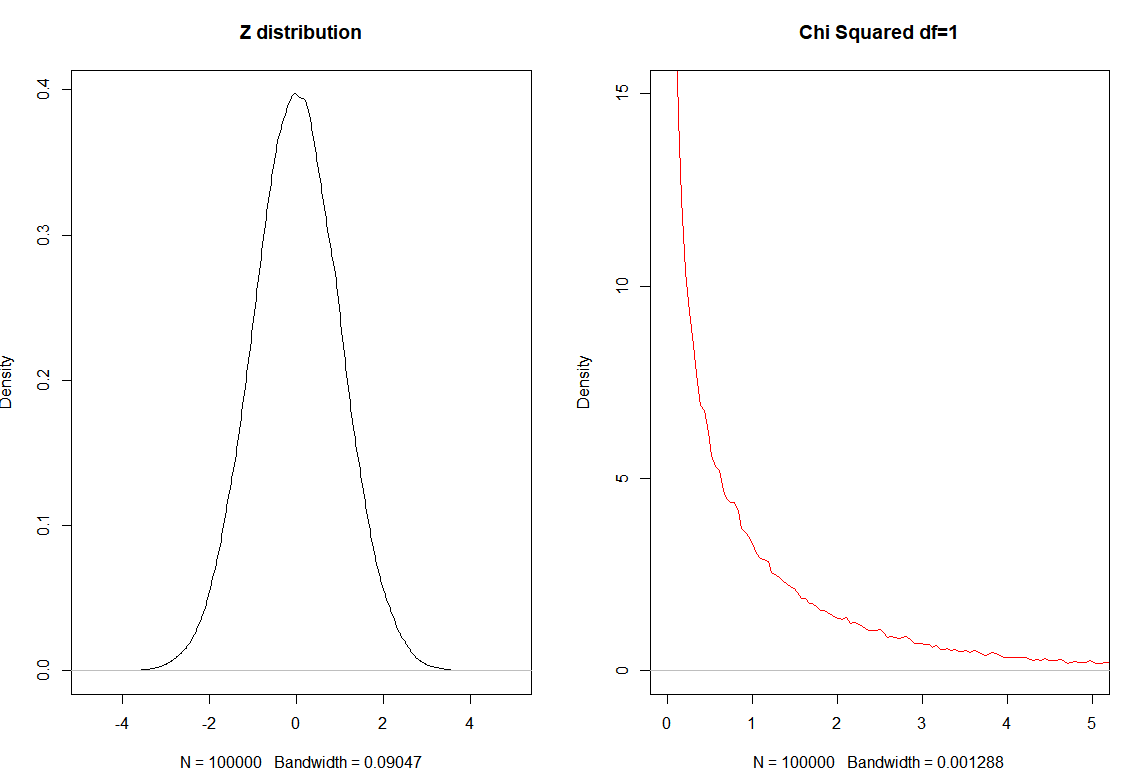
To create chi-squared distribution we start from Z-distribution.
\[Z \sim \mathcal N(0,1)\]And write:
\[Z_1^2 \sim \chi_1^2\]set.seed(0)
par(mfrow=c(1,2))
z = rnorm(10^5)
plot(density(z), main="Z distribution")
z2 = z^2
plot(density(z2, bw="SJ"),
main="Chi Squared df=1", col="red",
xlim=c(0,5), ylim=c(0,15))
Out:
Two degrees of freedom
How to get two degrees of freedom?
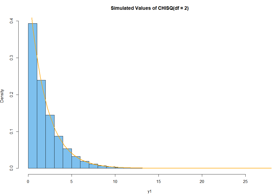
\[Z_1^2 + Z_2^2 \sim \chi_2^2\]Simple we square two $Z$ distributions and sum them up to get what is called Chi-Squared distribution with two degrees of freedom.
R code simulation for $\chi_2^2$
set.seed(0)
x1 = rnorm(10^6);  x2 = rnorm(10^6)
y1 = x1^2 + x2^2
hdr = "Simulated Values of CHISQ(df = 2)"
hist(y1, prob=T, br=30, col="skyblue2", main=hdr)
curve(dchisq(x, 2), add=T, lwd=2, col="orange")
In general to get $k$ degrees of freedom:
\[\sum_{i=1}^{n} Z_{i}^{2} \sim \chi_{n}^{2}\]Example: different degrees of freedom
Chi-Squared is actually gamma distribution with shape parameter $n/2$ and scale parameter $2$ is called the chi-square distribution with $n$ degrees of freedom. PDF is:
\[f(x)=\frac{1}{2^{n / 2} \Gamma(n / 2)} x^{n / 2-1} e^{-x / 2}, \quad x \in(0, \infty)\]Example: Let’s show what happens if we square 10^5 numbers from $\mathcal N(1,2)$ distribution and check for the mean of these numbers.
set.seed(0)
x1 = rnorm(10^5, mean=1, sd=2)
y1 = x1^2
mean(y1)
Out:
5.013841
This mean is $\mu + \sigma^2$ in other words. For the case where we have $Z$ distributions it is only $\sigma^2$.
Moments
For Variance $\mathbb V$ we have:
\[\mathbb V(Z) =\mathbb E[Z^2] - ( \mathbb E[Z])^2\]Since $\mathbb E[Z]=0$ we have:
\[\mathbb V(Z) =\mathbb E[Z^2]\]Finally, $\mathbb E[\chi_n]=n$, $\mathbb V(\chi_n) = 2n$
Goodness of fit test
Example: 100 people were interviewed who is the GOAT of Basketball? The answers were: 43 for Michael Jordan, 36 LeBron James and 21 for Kobe Bryant. Is there a GOAT at 5% level of significance?
$H_0$: There is no GOAT
$H_A:$ There is GOAT
If we would show that there is no enough evidence for the $H_0$ we could show there is a GOAT.
| Observations | Expected | |
|---|---|---|
| Jordan | 43 | 100/3 |
| LeBron | 36 | 100/3 |
| Briant | 21 | 100/3 |
| Total | 100 | 100 |
We first need to determine the degrees of freedom for this case $df=2$
When working with tables $df$ is total number of rows - 1.
Now we need to find the critical 5% level of significance for the Chi Squared distribution with 2 degrees of freedom.
This is the same as asking the question at what value of $x$ we have the qchisq (quartile function) reaches the 95%.
qchisq(.95,2)
Out:
5.99
Now we need to calculate the sum in R
n=100 # total number of observations
e = n/3 # expected
obs = c(43, 36, 21) # observed values
sum((obs-e)^2/e)
Out
[1] 2.8033333 0.2133333 4.5633333
[1] 7.58
Because 7.58 > $\chi_{crit}^2$ = 5.99 we reject the hypothesis and show that preferred (GOAT) player exist.
The same can be achieved with this:
chisq.test(obs)
Out:
	Chi-squared test for given
	probabilities

data:  obs
X-squared = 7.58, df = 2, p-value = 0.0226
Since p-value $<\alpha$ we reject $H_0$
Example: When will Novak Djokovic be GOAT if Federer and Nadal end their career with 20 GS?
tennis = c(20, 20, 35)
chisq.test(tennis)
Out:
	Chi-squared test for given
	probabilities

data:  tennis
X-squared = 6, df = 2, p-value = 0.04979
We show that for $\alpha=0.05$ Novak needs 35 GS titles to become a GOAT.
Note in here we have trinomial distribution and expected values > 5 and we can use the Chi-squared test.
Test For Independence
Example: Pearson Chi Square test also know as test of independence. Does the gender influence the favorite sport?
| Male | Female | |
|---|---|---|
| Football | 54 | 4 |
| Basketball | 46 | 39 |
| Volleyball | 21 | 80 |
$H_0$ hypothesis: There is no evidence gender provides preference to sports.
$H_A$ hypothesis: Gender provides sport preference.
To resolve and answer the question fast we will use this R code:
data <- matrix(c(54, 4, 46, 39, 21, 80), ncol=2, byrow=TRUE)
data <- as.table(data)
data
chisq.test(data)
Out:
	Pearson's Chi-squared test

data:  data
X-squared = 78.134, df = 2, p-value < 2.2e-16
Because p-value < 0.05 we reject the hypothesis $H_0$ and approve the alternative hypothesis.
But how this even works? We create total columns or marginal frequencies.
| Observed | Male | Female | Total |
|---|---|---|---|
| Football | 54 | 4 | 58 |
| Basketball | 46 | 39 | 85 |
| Volleyball | 21 | 80 | 101 |
| Total | 121 | 123 | 244 |
Now we need to calculate the expected frequencies assuming the column row independence.
| Expected | Male | Female | Total |
|---|---|---|---|
| Football | $\frac{58*121}{244}$ | $\frac{58*123}{244}$ | 58 |
| Basketball | $\frac{85*121}{244}$ | $\frac{85*123}{244}$ | 85 |
| Volleyball | $\frac{101*121}{244}$ | $\frac{101*123}{244}$ | 101 |
| Total | 121 | 123 | 244 |
Or after some calculus:
| Expected | Male | Female | Total |
|---|---|---|---|
| Football | 28.76 | 29.24 | 58 |
| Basketball | 42.15 | 42.85 | 85 |
| Volleyball | 50.08 | 50.91 | 101 |
| Total | 121 | 123 | 244 |
Now we need to calculate the sum (where $o$ means observed and $e$ expected value)
Which lead us to the $\chi^{2}=78.134$ which is greater than critical $\chi_{crit}^{2}=5.99$ for 2 degrees of freedom. To calculate the degrees of freedom we use the formula $df=(c-1)(r-1)$ where $c$ is the number of columns and $r$ is number of rows.
We came to the exact same conclusion that gender influences the favorite sport in this case.
De Moivre-Laplace theorem
You may asked yourself why Chi Squared distribution is used for Goodness of fit test?
Dealing with binomial distribution according to De Moivre-Laplace theorem when $n$ approaches $\infty$, having $p$ fixed the distribution of:
\[\frac{X-n p}{\sqrt{n p(1-p)}} \sim z\]In here the mean is $np$ and standard deviation is $\sqrt{n p(1-p)}$.
So if the conditions are meat binomial or multinomial distributions in general case will convert to Z-distribution.
Conclusion
To conclude the goodness of fit test is the same (or very similar) to the test for independence.
These tests are based on multinomial distributions and adhere to Z distribution when then the observed frequencies are big enough. Since we are interested in square metrics this is why we use Chi Square distribution.
…
tags: chisquared & category: r