Normal distribution in R | Examples

The Normal distribution functions

dnorm(x, mean = 0, sd = 1, log = FALSE)
pnorm(q, mean = 0, sd = 1, lower.tail = TRUE, log.p = FALSE)
qnorm(p, mean = 0, sd = 1, lower.tail = TRUE, log.p = FALSE)
rnorm(n, mean = 0, sd = 1)

If mean or sd are not specified they assume the default values of 0 and 1, respectively.

The normal distribution has density:

$f(x)=\Large \frac{1}{\sqrt{2 \pi \sigma^{2}}} e^{-\frac{(x-\mu)^{2}}{2 \sigma^{2}}}$

where $\mu$ is the mean of the distribution and $\sigma$ the standard deviation.

• dnorm gives the PDF density
• pnorm gives the CDF function
• qnorm gives the quantile function
• rnorm generates random deviates

For rnorm the length of the result is determined by n , and is the maximum of the lengths of the numerical arguments for the other functions.

For sd = 0 this gives the limit as sd decreases to 0, a point mass at $\mu$. sd < 0 is an error and returns NaN.

Example: Area under PDF based on condition

What is the percentage of students with the height > 170 if height is distributed normally $\mathcal N(150,20)$.

We can solve this very easy if we just know the percentage inside $[\mu-\sigma, \mu+\sigma]$ is ~68.2%.

Our percentage should be $(1-68.2)/2 \simeq 15.9$

In R we can integrate the dnorm to get the output.

integrate(dnorm, mean=150, sd=20, lower= 170, upper= Inf, abs.tol = 0)$value

Out

0.1586553

The same answer we get with:

1-pnorm(170, mean=150, sd=20)

dnorm is PDF, pnorm is CDF

Example: Random variable difference

Men have a mean height of 178cm with a standard deviation of 8cm. Womnen have a mean height of 170cm with a standard deviation of 6cm. Male and female heights are normally distributed. What is the probability that the woman is taller than the man?

$M = \mathcal N(178, 8), W = \mathcal N(170, 6)$

We are interested to find the new random variable $D = M-W$ of the difference.

To calculate:

$\mu_D = \mu_M -\mu_W=8 \ \sigma_D^2 = \sigma_M^2 +\sigma_W^2=100$

$\therefore \sigma_D = 10, \ D \sim \mathcal N(2,10)$

To calculate the probability woman is taller than man:

$\mathbb P(W \gt M) = \mathbb P(M-W < 0) = \mathbb P( D \lt 0)$

pnorm(0, mean=8, sd=10 )

Out:

0.211855398583397

Example:_ Combine two random variables_

Summer drives to work and back. The amount of fuel he uses follows a normal distribution:

To work: $\quad \mu_{W}=10 \mathrm{~L} \quad \sigma_{W}=1.5 \mathrm{~L}$

To home: $\quad \mu_{H}=10 \mathrm{~L} \quad \sigma_{H}=2 \mathrm{~L}$

If he has $25L$ of fuel and he intends to drive to work and back home. What is the probability that he runs out of fuel?

To calculate this we identify two random variables.

$W \sim \mathcal N(10, 1.5) \ H \sim \mathcal N(10, 2)
\therefore
B = \mathcal N(10+10, \sqrt{1.5^2+2^2}) = \mathcal N(20, 2.5)$

To run out of fuel we need $\mathbb P(B>25)$

1- pnorm(25, mean=20, sd=2.5 )

Out:

0.0227501319481792

Example: Calculate the $\sigma$ interval around the mean percentage

Get the percentage in area $[\mu - \sigma, \mu + \sigma ]$

bef <- pnorm(-1, mean=0, sd=1 )
bef
aft <- 1 - pnorm(1, mean=0, sd=1 )
aft
# finally
1-(bef+aft)

Out:

0.158655253931457
0.158655253931457
0.682689492137086

Example: A random variable $X \sim \mathcal N(37,7)$. Find the following probabilities:

• a) $\mathbb P(x<25)$
• b) $\mathbb P(x>42)$
• e) $\mathbb P(25<x<42)$

par(mfrow=c(1,2))
curve(dnorm(x,35,7), 10, 60, lwd=2, ylab="PDF", main="NORM(35,7)")
abline(h=0,col="green2"); abline(v = 25, col="red", lty="dashed")
curve(dnorm(x,35,7), 10, 60, lwd=2, ylab="PDF", main="NORM(35,7)")
abline(h=0,col="green2"); abline(v = 42, col="blue", lty="dashed")

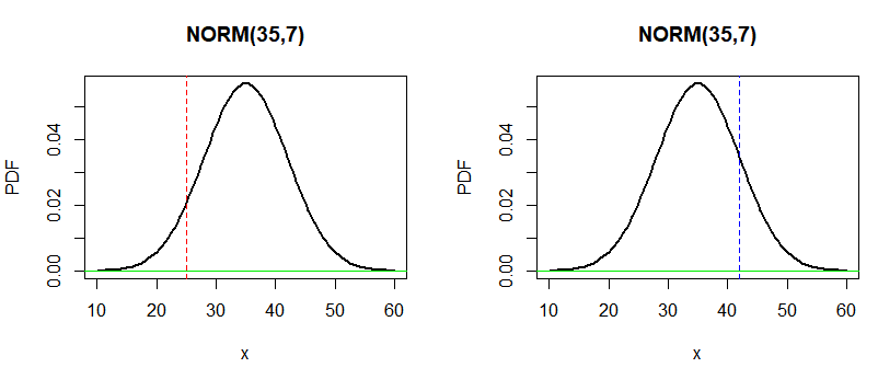
For the a) case we can integrate dnorm where $x<25$

integrate(dnorm, mean=35, sd=7, lower= -Inf, upper=25, abs.tol = 0)$value

Out:

0.07656373

Exact same result would be to call pnorm(25, mean=35, sd=7 )

b) Again we can integrate but different region from $x>42$

integrate(dnorm, mean=35, sd=7, lower=42, upper=Inf, abs.tol = 0)$value

Out:

0.1586553

The same result we may get using the pnorm function:

1-pnorm(42, mean=35, sd=7)

par(mfrow=c(1,1))
curve(dnorm(x,35,7), 10, 60, lwd=2, ylab="PDF", main="NORM(35,7)")
abline(h=0,col="green2"); 
abline(v = c(25,42), col="darkgreen", lty="dashed")

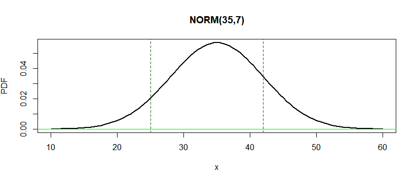
c) To solve the region $24<x<42$ we may integrate dnorm again:

integrate(dnorm, mean=35, sd=7, lower=25, upper=42, abs.tol = 0)$value

Out:

0.764781

Or we may use:

1 - pnorm(25, mean=35, sd=7) -(1-pnorm(42, mean=35, sd=7))

Example: Product of two random variables

If we have two random variables $X \sim \mathcal N(\mu_1, \sigma_1)$ and $Y \sim \mathcal N(\mu_2, \sigma_2)$

Then the effective $\mu$ and $\sigma$ of the product would be:

Based on the fact Gaussian exponents are quadratic: