t-distribution | Examples

It was developed by English statistician William Gosset when he worked for Guinness (famous for world records).

Guinness didn’t want the competitors to hire statisticians knowing how impactful and useful they are.

Gosset published a t-distribution paper under the pseudonym “Student”.

T-distribution PDF:

We use t-distribution when the number of samples is relatively small, say $n<30$ when we don’t have the $\sigma$ SD of the population. Instead we use $S$ standard deviation of the sample.

If we would have $\sigma$ we would probably use z-distribution.

How z-distribution and t-distribution match

t.values <- seq(-4,4,.1)
plot(x = t.values,y = dnorm(t.values,sd=1), lty = "dotted", type="l", col="black", ylim = c(0,.4), xlab = "x", ylab = "y")
lines(x = t.values,y = dt(t.values,df=3), type = "l", col="blue")
lines(x = t.values,y = dt(t.values,df=2), type = "l", col="red")
lines(x = t.values,y = dt(t.values,df=1), type = "l", col="green2")

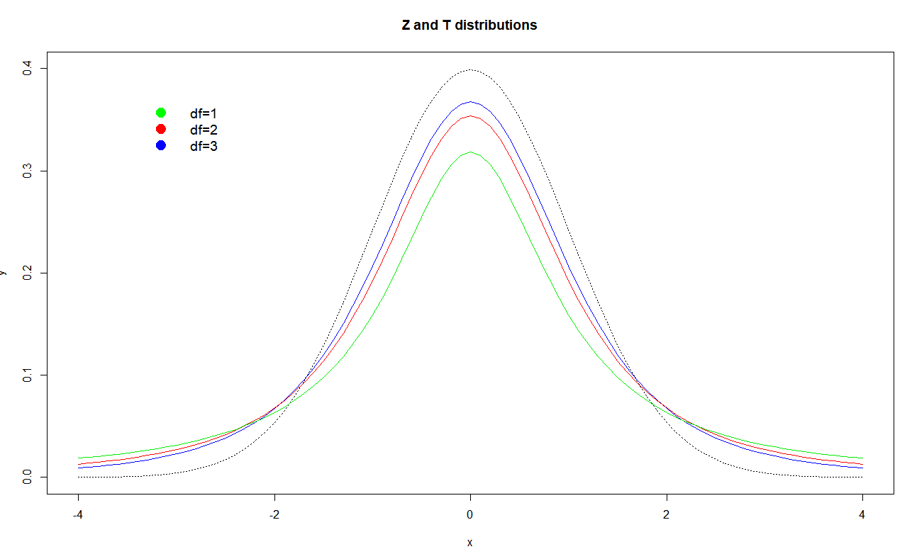
The legend shows t-distributions with different degrees of freedom and the dotted black line is z-distribution.

Finally the $df=29$ reflects the sample $n=30$.

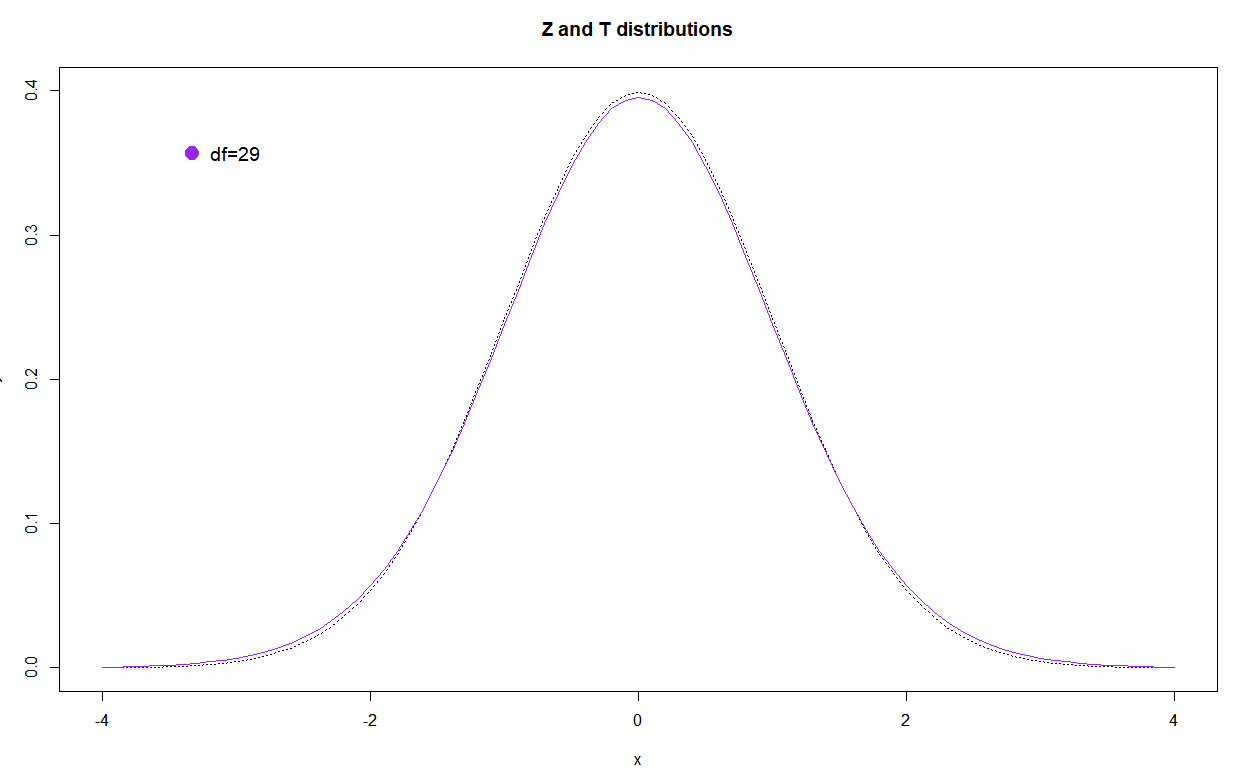
You can note how close this is to the z-distribution.

The t-distribution functions in R

dt(x, df, ncp, log = FALSE)
pt(q, df, ncp, lower.tail = TRUE, log.p = FALSE)
qt(p, df, ncp, lower.tail = TRUE, log.p = FALSE)
rt(n, df, ncp)

Since $S$ brings uncertainty, unless $n$ is big enough (where we usually assume $\sigma \approx S$) we decrease the degrees of freedom for the t-distribution:

Example: Heights of basketball players are: 201, 196, 209, 188, 205. Find 95% confidence interval of height.

With $n=5$ samples we have $df=4$ so we can calculate $t$, $\bar X$ and all we need to set the confidence interval:

n<-5
z <- c(201, 196, 209, 188, 205)
summary(z)
mean(z)
sd(z)
t = qt(0.975,df=n-1)
t

Out:

> summary(z)
   Min. 1st Qu.  Median    Mean 3rd Qu.    Max.
  188.0   196.0   201.0   199.8   205.0   209.0
> mean(z)
[1] 199.8
> sd(z)
[1] 8.167007
> t = qt(0.975,df=n-1)
> t
[1] 2.776445

Confidence interval is:

$\bar X \pm t \frac{S}{\sqrt{n}}$

lower <- mean(z)-sd(z)*t/sqrt(n)
upper <- mean(z)+sd(z)*t/sqrt(n)
print(lower)
print(upper)

Out:

> print(lower)
[1] 189.6593
> print(upper)
[1] 209.9407

Now we can say the 95% confidence interval for the player height is $(189.66, 209.94)$