Statistics Interview Questions

In here I will ask and answer many questions from statistics.
Table of Contents:
- What is regression?
- What is Information?
- What is entropy?
- How to maximize the entropy?
- 12 balls in a bin entropy
- What is cross-entropy?
- Cross-Entropy as Loss Function
- Probability of an Event
- Bayesian low
- Bayesian spam filer (naive bayes)
- Problem of the Naive Bayes model
- The Law of Large Numbers (LLN)
- Central Limit Theorem
- What is SE (Standard Error)?
- What is called
erfin statistics (math)? - Draw normal PDF. What is below the curve?
- Draw normal CDF, what is below the curve?
- What is characteristic function?
- What is hypothesis testing?
- What is T-testing?
- What is power (statistics)?
- What is p-hacking?
- What is p-value?
- Books and materials
What is regression?
In statistics regression is an approach to find the relationship between variables and use that for prediction.
What is Information?
Claude Shannon defined information as:
$I(x) = -log₂P(x)$, where $P(x)$ is probability of occurrence of the variable $x$.
If $P(x)=1$, or if we are absolutely certain:
$I(x)=-log₂1=0$, there is no information.
There is information if $P(x)<1$ (probability of the occurrence is less than 1).
This is why Shannon defined: Information quantifies the uncertainty in one single event.
The more we are uncertain of the more information.
In a fair coin toss game probability for the coin head is 0.5. Let’s calculate the information.
$I(x) = -log₂P(x)=-log₂\frac12=1$
Information is 1 bit.
For the rolling dice problem the probability we get 1, is $\frac 16$.
The information we will get 1 will then be:
$I(x) = -log₂P(x)=-log₂\frac16=2.58491$
This tells us the information in bits.
If we would have $P(x)=0$,
$I(x) = -log₂P(x)=-log₂0=∞$. Information would be = $∞$ bits.
What is entropy?
Let’s consider a simple 9 balls bin: {2 red, 3 green, 4 blue}. You pick one ball at random. What is the expected amount of information you will receive with a single pick?
We can say ball picking is random variable $X$.
A random variable is a variable whose possible values have an associated probability distribution and sample space from where the values are taken.
We need the entropy $E[X]$ of this random variable.
Don’t confuse entropy of a random variable with the expected value of the random value $\mathbb E[X]$.
First we align probabilities and associated information values:
$P(R) = \frac29$ => $I(R)=-log₂\frac29$
$P(G) = \frac39$ =>$I(G)=-log₂\frac39$
$P(B) = \frac49$ => $I(B)=-log₂ \frac49$
Entropy is weighted sum of all the information, where the weights are the corresponding probabilities.
$Entropy(X) = -[\frac29\cdot log₂\frac29 + \frac39 \cdot log₂ \frac39 + \frac49 \cdot log₂\frac49]$ = 1.53 bits.
For a single ball entropy $E[X]$=1.53 bits.
Information entropy is typically measured in bits (or “shannons”) corresponding to base 2 in the above equation.
If we use $log_e$ these will be natural units or nats.
If we mesure it with $log_{10}$ these are called:
- dits
- bans or
- hartleys
Instead of writing $E[X]$ for the entropy of $X$ more frequent notation is to use $H[X]$.
How to maximize the entropy?
For the case with 9 balls and 3 different colors we should have 3 balls of each color: 3 red, 3 green, and 3 blue balls.
L = {3 red, 3 green, 3 blue}
$Entropy(X) = -[\frac39\cdot log₂\frac39 + \frac39 \cdot log₂ \frac39 + \frac39 \cdot log₂\frac39]$ = 1.58 bits
The results is equal to $log₂3$
Entropy will be maximized if uncertainty of any element is maximized.
12 balls in a bin entropy
Case when we have 12 balls in a bin, equal number of the same colors.
L1 = {12}, $E(X) = log_2 1$
L2 = {6,6}, $E(X) = log_2 2$
L3 = {4,4,4}, $E(X) = log_2 3$
L4 = {3,3,3,3} $E(X) = log_2 4$
L5 = {2,2,2,2,2,2} $E(X) = log_2 6$
L6 = {1,1,1,1, 1,1,1,1, 1,1,1,1} $E(X) = log_2 12$
We may note entropy will increase if there are more color groups.
What is cross-entropy?
Cross-entropy measures the relative entropy between two probability distributions L1 and L2 over the same set of events.
Let’s consider two bins with the labels:
L1 = {2 red, 3 green, 4 blue} and L2 = {3 red, 3 green, 3 blue}
$H(L1, L2) = -[\frac 29 \cdot log₂\frac 39 + \frac39\cdot log₂ \frac39 + \frac 49 \cdot log₂ \frac 39]$
$H(L1, L2) = 1.58$
The results is equal to $log₂3$
Cross-Entropy as Loss Function
In machine learning we use cross-entropy as a loss function. How this works?
If we have classes: C1, C2, C3.
Let L1 be the true label distribution and L2 be the predicted label distribution.
Let the only label for one sample is C2 and our classifier predicts probabilities for C1, C2, C3 as (0.15, 0.60, 0.25).
Cross-entropy $H(L1, L2)$ will be:
$H(L1, L2) = -[0 * log₂(0.15) + 1 * log₂(0.6) + 0 * log₂(0.25)] = 0.736$
On the other hand, if our classifier is more confident and predicts probabilities as (0.05, 0.90, 0.05), we would get cross-entropy value is 0.152, which is lower than the above example.
Now our aim is to maximize the cross-entropy in this case.
Probability of an Event
We use $P(E)$ to express probability associated with an event $E$.
If we have two events and following is true: $P(E1,E2) = P(E1)\cdot P(E2)$
Then we say events $E1$ and $E2$ are independent.
For instance flipping a coin. $E1$ is the first flip, $E2$ is the second flip. If the outcome of the event $E1$ is either head or tail this doesn’t have impact to the second flip outcome $E2$.
But if we define the event $E2$ different, saying $E2$ is at least one head in two flips, then $E1$ and $E2$ are dependent.
$P(E2,E1) = P(E2∣E1)\cdot P(E1)$
This reverts to independent case when: $P(E2∣E1)= P(E2)$
We could rewrite the dependent form as:
$P(E2∣E1) = P(E2,E1)/P(E1)$
~~
Example: Flipping the coin.
What is probability of both heads in two consecutive flips if at least one flip is head?
Probability of first head is $\frac12$. Probability of two heads is $\frac14=\frac12 \cdot \frac12$, because second head is independent of first, and we have independent events.
However, now we have:
$P(B)$ - both
$P(L)$ - at least one
$P(B ∣ L)=P(B, L)/P(L)$
$P(L)=\frac34$ because {HH, HT, TH, TT}
$P(B ∣ L)=P(B)/P(L)={\frac14 / \frac34 = \frac 13}$
~~
Bayesian low
Expressed as:
$P(S∣M) = \Large {P(M∣S) \cdot P(S) \over P(M)}$
Replacement:
$P(M)= P(S)P(M∣S) + P( \neg S)P(M∣ \neg S)$
Leads to:
$P(S∣M) = \Large {P(M∣S)\cdot P(S) \over P(S)P(M∣S) + P( \neg S)P(M∣ \neg S)}$
~~
Example: Rain.
Probability that it will rain on Sunday is 40%. If it rains on Sunday probability it will rain on Monday is just 10%, but without rain on Sunday probability it will rain on Monday is high and equals 80%.
What are the chances it will rain on Monday? If it rained on Monday, what is the probability it rained on Sunday?
We know:
$P(S)=0.4$
$P(M∣S)=0.1$
$P(M∣\neg S)=0.8$
We conclude:
$P(\neg S)=0.6$
$P(\neg M∣S)=0.9$
$P(\neg M∣\neg S)=0.2$
To calculate the $P(M)$ we use the replace rule:
$P(M)= P(S)P(M∣S) + P( \neg S)P(M∣ \neg S)$
$P(M)= 0.4 \cdot 0.1 + 0.6 \cdot 0.8 = 0.52$
Then we use Bayesian rule:
$P(S∣M) = {P(M∣S)*P(S) \over P(M)}$
$P(S∣M) ={0.1 \cdot 0.4 \over 0.52}=0.0769$
~~
Bayesian spam filer (naive bayes)
We can use the Bayesian formula:
\[P(spam∣words) = {P(words∣spam)* P(spam) \over P(words)}\]To train the bayesian filtering model with many words $w_1, w_2, …, w_n$.
Bayesian filtering can predict if a message is spam based on the words given.
It works based on the fact that some words have a higher chance of appearing in spam messages than in normal ones.
Inside scikit-learn python package there is a BernoulliNB model that implements the Naive Bayes algorithm.
~~
Example: Simple filter for the word viagra
We know half of all spam messages have the word viagra and 1% of non spam messages have the same word, would would be probability that the email with the word viagra is spam?
Let we use $S$ for message is spam. Let $V$ is the event when email contains the word viagra.
Then Bayes’s theorem tells us that the probability that the message is spam conditional on containing the word viagra is:
$P(S∣V) = \Large {P(V∣S)\cdot P(S) \over P(V∣S)\cdot P(S)+P(V∣\neg S)\cdot P(¬S)}$
Numerator meaning: message is spam and contains viagra
Denominator meaning: probability that a message contains viagra or $P(V)$ written in another form.
This calculation is simply representing the proportion of viagra messages that are spam.
If we would have collection of email we know are spam, and collection of email that are not spam, then we can know calculate $P(V∣S)$ and $P(V∣ \neg S)$
We can assume equal case $P(S) = P(\neg S) = 0.5$,
\[P (S∣ V) = {P( V∣ S) \over P(V, S) + P (V∣ \neg S)}\]This then lead to the following conclusion:
If we know $P(V∣S)=0.5$, half of all spam messages have the word viagra, and 1% of non spam messages have the same word $P(V∣\neg S)=0.01$, then the then the email is spam if the word viagra is in it is: $\frac{0.5}{0.51} =0.98$.
~~
Problem of the Naive Bayes model
The Naive Bayes is having a constraint. Words inside email $w_1, w_2, … ,w_n$ are independent of one another. There is only a conditional on a message being spam or not. This may explain why there are better approaches for filtering spam.
The Law of Large Numbers (LLN)
Consider some process like rolling a dice.
Then you may note the average of the observed values in the long run will be closer to the expected value.
When rolling a fair dice, with the expected outcomes {1, 2, 3, 4, 5, 6} the expected value is 3.5:
(1 + 2 + 3 + 4 + 5 + 6) / 6 = 3.5.
We can reach that number with large number of observations. This is LLN.
Central Limit Theorem
The Central Limit Theorem say for any distribution if we take multiple samples of equal size, sample means will have the normal distribution as long as the sample size is greater than 30 samples.
Or:
Given a sufficiently large sample size, the sampling distribution of the mean for a variable will approximate a normal distribution regardless of that variable’s distribution in the population.
What is SE (Standard Error)?
The Standard Error (SE) considers taking multiple n-samples from probability distribution, and recording of the means obtained in repeat. For Gauss or normal distribution it should be: $\Large \frac {\sigma }{\sqrt {n}}$
where: $\Large σ$ is the standard deviation of the population, $\Large n$ is number of observations of the sample.
What is called erf in statistics (math)?
This is a Gauss error function connected to Gauss or normal distribution.
In Python you can find it under math.erf. The property of this function it goes from -1, to 1. The function has no singularities except at negative infinity and positive infinity. You can define it as:
The erf graph looks like this:
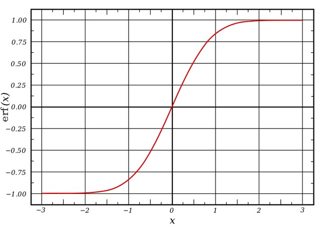
Interpretation:
For a random variable $Y$ that is normally distributed with $\mu=0$, $\sigma^2=0.5$, erf$(x)$ is the probability that $Y$ falls in the range $[−x, x]$.
Draw normal PDF. What is below the curve?
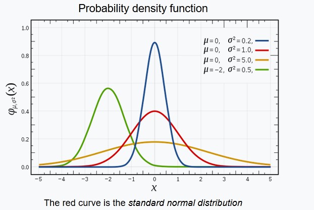
The total area under the curve for any PDF (Probability Distribution Function), not just for normal is equal to 1. This curve represents the random variable distribution.
Draw normal CDF, what is below the curve?
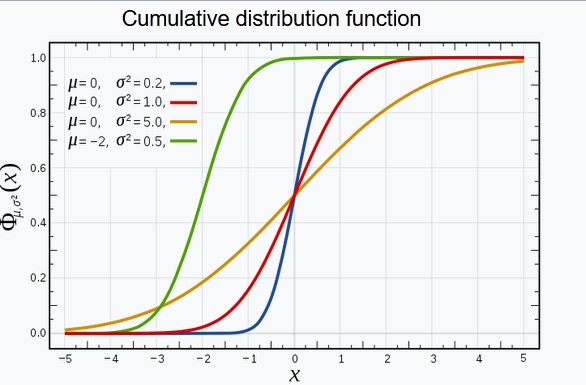
Cumulative Distribution Function (CDF) represents how fast the area below PDF reaches 1.
What is characteristic function?
The characteristic function provides an alternative way for describing a random variable, or in other words it is a function that completely describes probability distribution. You can find for instance standard normal distribution characteristic function which is simply the Fourier transform.
What is hypothesis testing?
A hypothesis test is a formal approach for evaluating a research question.
We analyze the data to evaluate if hypothesis is true. For instance, whether man or women are promoted more often.
Null hypothesis would be, gender do not influence promotion recommendation. In this case we should evidence gender rates are about the same.
Alternative hypothesis would be man are favored (or woman are favored).
What is T-testing?
T-test is any statistical hypothesis test in which the test statistic follows Student’s t-distribution under the null hypothesis.
A t-test is most commonly applied when the test statistic would follow a normal distribution.
What is power (statistics)?
The power of a binary hypothesis test is the probability that the test rejects the null hypothesis when a specific alternative hypothesis is true.
The statistical power ranges from 0 to 1, and as statistical power increases, the probability of making a type II error decreases.
What is p-hacking?
p-hacking (fishing, snooping) is the misuse of data analysis to find patterns in data that can be presented as statistically significant, thus dramatically increasing and understating the risk of false positives.
False positive is a test result which wrongly indicates that a particular condition or attribute is present.
The process of p-hacking assumes investigating the p-value. p-hacking is common belief that p-value has huge impact on validity of the experiments. The problem is this seams not to be always true.
What is p-value?
p-value is:
- number between 0 and 1.
- possible the evidence against a null hypothesis.
- the smaller the p-value, the stronger the evidence
A p-value less than 0.05 is statistically significant.
It indicates strong evidence against the null hypothesis.
If p-value < 0.05 We may reject the null hypothesis, and accept the alternative hypothesis.
Books and materials
OpenIntro Statistics
This is a special online book with many topics about statistics and direct link to YouTube videos.
Interesting topics:
- Probability (special topic).
- The basic principles of probability.
- Distributions of random variables.
- Introduction to the normal model and other key distributions.
- Foundations for inference.
- General ideas for statistical inference
- Inference for numerical data.
- Inference for one or two sample means using the t-distribution, and also comparisons of many means using ANOVA.
Modern analyst (modernanalyst.com)
Modern analyst is a great website covering interview questions: Search Google on “site:https://www.modernanalyst.com/Careers/InterviewQuestions/”
StatsModels
Statistical models is very advanced GitHub repo for statistical modeling and econometrics in Python. You can reach the documentation here.
It is a complement to scipy for statistical computations including descriptive statistics and estimation and inference for statistical models.
OpenStax Introductionary Statistics
This is a great textbook you can download from openstax.org website.
…
tags: questions - probability - theory & category: statistics