Pandas basic operations

Pandas is a a great package for data analysis. In pandas you will deal with Series and DataFrames.
Table of contents:
- Loading pandas
- The DataFrame and the Series object
- Create the DataFrame using the constructor
- Load the DataFrame multiple ways
- Get info about the DataFrame
- Column types
- Read and write data
- Add and remove columns
- Indexing
- Boolean indexing (masking)
- map and apply
- groupby
- Check the version
Loading pandas
To load the pandas library you just execute:
import pandas as pd
I never saw any other alias for pandas except pd.
Pandas run on numpy. Still we may load the Numpy alias as well.
import numpy as np
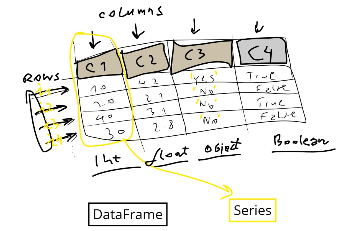
The DataFrame and the Series object
DataFrame in pandas is the second name for the table with named columns and named rows.
Series object in pandas represent a single column. Alternative name for the column is feature.
Alternative name for any row is an instance, or an observation.
Create the DataFrame using the constructor
We covered already the Pandas load data, and now we will dig into operations we can call on a DataFrame or Series.
Let’s create single empty DataFrame first filled with NaN values:
Example:
df = pd.DataFrame(index=range(14),columns=range(7))
print(df)
Output:
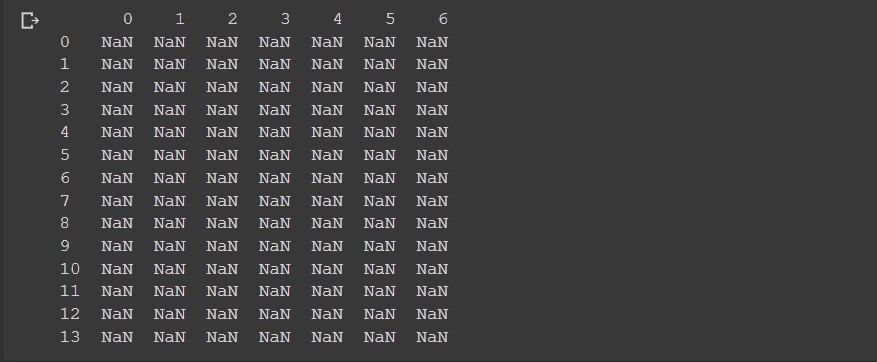
Here we set the 7 columns and 14 rows. Note how in python pandas the start index is always 0.
To create a DataFrame you may also provide the column names and row index names.
Example:
import pandas as pd
df = pd.DataFrame(index=['a', 'b', 'c'], columns=['time', 'date', 'name'])
print(df)
print(df.values)
Output:
  time date name
a  NaN  NaN  NaN
b  NaN  NaN  NaN
c  NaN  NaN  NaN
[[nan nan nan]
 [nan nan nan]
 [nan nan nan]]
Let’s create a mini DataFrame based on a simple Python matrix:
Example:
df= pd.DataFrame([[1,2,3], ['a', 'b', 'c']])
print(type(df))
df
Output:
  0   1   2
0   1   2   3
1   a   b   c
As we can see, we have two rows 0,1 and three columns 0,1,2.
Let’s create a DataFrame from named columns:
Example:
d = {'col1': [1, 2], 'col2': [3, 4]}
df = pd.DataFrame(d)
df
Output:
   col1  col2
0  1     3
1  2     4
This time column names are ‘col1’ and ‘col2’.
Let’s create both named rows and columns:
Example:
df = pd.DataFrame([[1, 2, 3],[4, 4, 4],[5, 6, 7]],
                  index=['i1', 'i2', 'i3'],
                  columns=['a', 'b', 'c'])
df
Output:
  a   b   c
i1  1   2   3
i2  4   4   4
i3  5   6   7
Load the DataFrame multiple ways
There are several cases where we load the DataFrame from text, or from textual file or from CSV file or from remote URL.
Almost always we use the read_csv method.
Example:
import io

s='''Person,Age,Single
0,John,24.0,False
1,,NaN,None
2,Lewis,21.0,True
3,John,33.0,True
4,Myla,26.0,False'''

df=pd.read_csv(io.StringIO(s),
                sep=r',',
                engine='python',
                keep_default_na=True,
                na_values=['NaN', None,' '],
                encoding="iso-8859-1")

df
Output:
  Person  Age   Single
0   John  24.0  False
1   NaN   NaN   NaN
2   Lewis   21.0  True
3   John  33.0  True
4   Myla  26.0  False
In here the , was the separator.
Note how we set the na_values. Anything inside that array will be treated as NaN.
NaN value corresponds to np.nan.
Let’s try another separator:
Example:
import io
s='''"";"Gender";"FSIQ";"VIQ";"PIQ";"Weight";"Height";"MRI_Count"
"1";"Female";133;132;124;"118";"64.5";816932
"2";"Male";140;150;124;".";"72.5";1001121
"3";"Male";139;123;150;"143";"73.3";1038437
"4";"Male";133;129;128;"172";"68.8";965353
"5";"Female";137;132;134;"147";"65.0";951545
'''
df=pd.read_csv(io.StringIO(s),
                sep=r';',
                engine='python',
                keep_default_na=True,
                na_values=['NaN', None,' '],
                index_col=0,
                encoding="iso-8859-1")
df
Output:
  Gender  FSIQ  VIQ   PIQ   Weight  Height  MRI_Count
1   Female  133   132   124   118   64.5  816932
2   Male  140   150   124   .   72.5  1001121
3   Male  139   123   150   143   73.3  1038437
4   Male  133   129   128   172   68.8  965353
5   Female  137   132   134   147   65.0  951545
In here we used a different separator ; and we used index_col=0, meaning the very first column will be the index.
Here is another example where the separator is multiple spaces.
Example:
import io
s='''Person   Age  Single
  0    John  24.0   False
  1    Myla   NaN    True
  2   Lewis  21.0    True
  3    John  33.0    True
  4    Myla  26.0   False'''

df =pd.read_csv(io.StringIO(s),
                sep=r'\s{2,}', # 2 or more spaces
                engine='python',
                encoding="iso-8859-1")
df
Output:
  Person  Age   Single
0   John  24.0  False
1   Myla  NaN   True
2   Lewis   21.0  True
3   John  33.0  True
4   Myla  26.0  False
Note we used so far the pandas read_csv method. We will use it again to read from the remote URL.
Example:
url = "https://archive.ics.uci.edu/ml/machine-learning-databases/iris/iris.data"
names = ['sepal-length', 'sepal-width', 'petal-length', 'petal-width', 'class']
df = pd.read_csv(url, names=names)
df
Output:
  sepal-length  sepal-width   petal-length  petal-width   class
0   5.1   3.5   1.4   0.2   Iris-setosa
1   4.9   3.0   1.4   0.2   Iris-setosa
2   4.7   3.2   1.3   0.2   Iris-setosa
3   4.6   3.1   1.5   0.2   Iris-setosa
4   5.0   3.6   1.4   0.2   Iris-setosa
...   ...   ...   ...   ...   ...
145   6.7   3.0   5.2   2.3   Iris-virginica
146   6.3   2.5   5.0   1.9   Iris-virginica
147   6.5   3.0   5.2   2.0   Iris-virginica
148   6.2   3.4   5.4   2.3   Iris-virginica
149   5.9   3.0   5.1   1.8   Iris-virginica
Get info about the DataFrame
Let’s load the DataFrame as in the previous example:
url = "https://archive.ics.uci.edu/ml/machine-learning-databases/iris/iris.data"
names = ['sepal-length', 'sepal-width', 'petal-length', 'petal-width', 'class']
df = pd.read_csv(url, names=names)
df
To get the info from the DataFrame we call:
df.info()
Output:
<class 'pandas.core.frame.DataFrame'>
RangeIndex: 150 entries, 0 to 149
Data columns (total 5 columns):
sepal-length    150 non-null float64
sepal-width     150 non-null float64
petal-length    150 non-null float64
petal-width     150 non-null float64
class           150 non-null object
dtypes: float64(4), object(1)
memory usage: 6.0+ KB
As you can see df.info() method explains the columns. If the number of columns is large, we can call first:
df.columns
to get the list of columns, and then for instance:
df['sepal-length'].describe()
To get info on a particular column. Mentioned method describe() can also provide statistical info for the DataFrame:
df.describe()
Output:
  sepal-length  sepal-width   petal-length  petal-width
count   150.000000  150.000000  150.000000  150.000000
mean  5.843333  3.054000  3.758667  1.198667
std   0.828066  0.433594  1.764420  0.763161
min   4.300000  2.000000  1.000000  0.100000
25%   5.100000  2.800000  1.600000  0.300000
50%   5.800000  3.000000  4.350000  1.300000
75%   6.400000  3.300000  5.100000  1.800000
max   7.900000  4.400000  6.900000  2.500000
It would be good to know the most valuable methods we can call on Series next:
Examples:
df['sepal length'].value_counts()
df['sepal length'].unique()
df['sepal length'].nunique()
value_counts will return data for the histogram (frequency per unique values):
5.0    10
6.3     9
5.1     9
6.7     8
5.7     8
5.5     7
5.8     7
6.4     7
6.0     6
4.9     6
6.1     6
5.4     6
5.6     6
6.5     5
4.8     5
7.7     4
6.9     4
5.2     4
6.2     4
4.6     4
7.2     3
6.8     3
4.4     3
5.9     3
6.6     2
4.7     2
7.6     1
7.4     1
4.3     1
7.9     1
7.3     1
7.0     1
4.5     1
5.3     1
7.1     1
Name: sepal-length, dtype: int64
unique will return just the unique values:
array([5.1, 4.9, 4.7, 4.6, 5. , 5.4, 4.4, 4.8, 4.3, 5.8, 5.7, 5.2, 5.5,
       4.5, 5.3, 7. , 6.4, 6.9, 6.5, 6.3, 6.6, 5.9, 6. , 6.1, 5.6, 6.7,
       6.2, 6.8, 7.1, 7.6, 7.3, 7.2, 7.7, 7.4, 7.9])
nunique will return the the number of unique values:
35
Statistical methods on a DataFrame
df.describe()
df.mean()
df.median()
df.max()
df.min()
df.count()
df.std()
df.corr()
To get more feedback on each method run help, for instance:
help(df.mean)
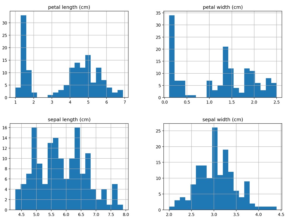
Histogram
We mentioned the histogram. Let’s show how histogram is called in pandas.
For this experiment I will load the iris dataset from URL and call hist().
from sklearn.datasets import load_iris
import pandas as pd
data = load_iris()
df = pd.DataFrame(data.data, columns=data.feature_names)
fig,ax = plt.subplots(dpi=153, figsize=(12,9))
df.hist(ax=ax, bins=20)
Output:
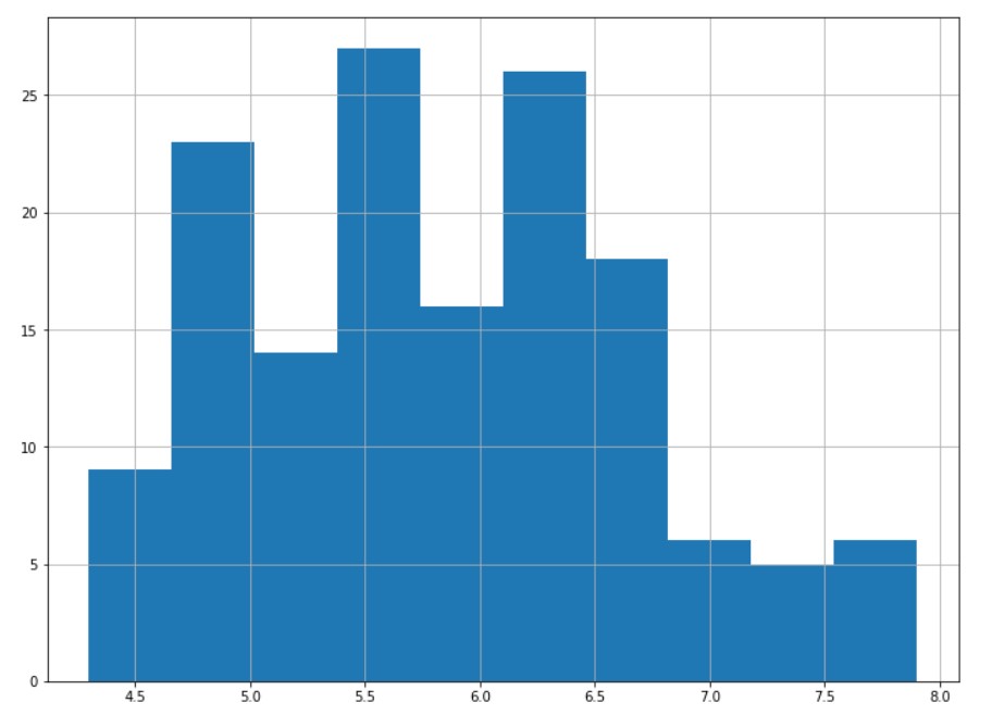
If we plan to create just a single column histogram we will call:
df[df.columns[0]].hist(figsize=(12,9))
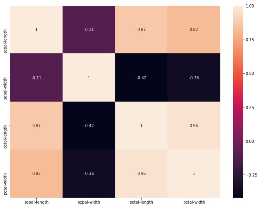
Correlation
Works simple as:
df.corr()
Output:
  sepal length (cm)   sepal width (cm)  petal length (cm)   petal width (cm)
sepal length (cm)   1.000000  -0.117570   0.871754  0.817941
sepal width (cm)  -0.117570   1.000000  -0.428440   -0.366126
petal length (cm)   0.871754  -0.428440   1.000000  0.962865
petal width (cm)  0.817941  -0.366126   0.962865  1.000000
It would be nice to show the correlation in visual way:
from matplotlib import pyplot as plt
import seaborn as sns
plt.figure(figsize=(25,10))
ax = sns.heatmap(df.corr(), annot=True)
bottom, top = ax.get_ylim()
ax.set_ylim(bottom + 0.5, top - 0.5)
There are two major correlation types in use:
- Pearson
- Spearman
Pearson measures linear correlation and Spearman measures rank order correlation. There is also Kendall correlation.
You can specify the correlation type using the method parameter: df.corr(method='spearman').
You can use Pearson just in specific cases, else use Spearman type.
For the Pearson correlation both variable:
- should be normally distributed
- should have straight line relationship (linearity)
- data should be equally distributed about the regression line (homoscedasticity).
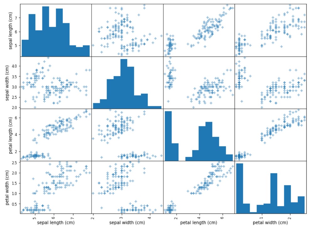
Scatter matrix
To create scatter matrix you would use this code:
from pandas import plotting
sm=plotting.scatter_matrix(df, figsize=(12,9), marker='+', hist_kwds={'bins':10})
Column types
There are just a couple most frequent column types in pandas.
- Numerical
- float
- int
- Categorical
- string (read:object)
- ordered string
- boolean
Ordered strings are strings with some grade semantics:
- elementary school
- middle school
- university
- after I graduate …
Often we have just two values for the single column like: ‘No’,’Yes’ or 0, 1 or False, True.
Read and write data
First we create a 100x100 DataFrame.
import numpy as np
import pandas as pd
df = pd.DataFrame(np.random.rand(100, 100))
The best methods to add a single value to a DataFrame are iat and at:
%timeit df.iat[50,50]=50
%timeit df.at[50,50]=50
%timeit df.iloc[50,50]=50
%timeit df.loc[50,50]=50
Methods iat and iloc are using column index number while method at and loc are using column names. For the previous example these are the same.
The best methods to set multiple values to a DataFrame are iloc and loc.
To read single value we would use: iat or at and to read multiple values we would use iloc and loc.
Add and remove columns
If we use the previous iris DataFrame we may create two new columns:
Example:
df['slen_plus_plen']=df['sepal-length']+df['petal-length']
df['auto'] = np.where(df['petal-width']==0.2, 'Good', 'Bad')
df
To drop a column we would use drop method:
df=df.drop(columns=['slen_plus_plen'])
Indexing
Pandas indexing means getting the elements from the DataFrame.
In here we show just the two columns
df[['sepal-length', 'sepal-width']]
This is equivalent to (will have the same output):
df.loc[:,['sepal-length', 'sepal-width']]
  sepal-length  sepal-width
0   5.1   3.5
1   4.9   3.0
2   4.7   3.2
3   4.6   3.1
4   5.0   3.6
...   ...   ...
145   6.7   3.0
146   6.3   2.5
147   6.5   3.0
148   6.2   3.4
149   5.9   3.0
To get just the first two rows and all columns:
df.loc[[0,1],:]
  sepal-length  sepal-width   petal-length  petal-width   class   auto
0   5.1   3.5   1.4   0.2   Iris-setosa   Good
1   4.9   3.0   1.4   0.2   Iris-setosa   Good
Boolean indexing (masking)
This would return the values based on condition:
df[df['petal-length']>5]
This will return values based on two conditions:
df[(df['petal-length']>5) & (df['sepal-length']>7)]
Output:
sepal-length  sepal-width   petal-length  petal-width   class   auto
102   7.1   3.0   5.9   2.1   Iris-virginica  Bad
105   7.6   3.0   6.6   2.1   Iris-virginica  Bad
107   7.3   2.9   6.3   1.8   Iris-virginica  Bad
109   7.2   3.6   6.1   2.5   Iris-virginica  Bad
117   7.7   3.8   6.7   2.2   Iris-virginica  Bad
118   7.7   2.6   6.9   2.3   Iris-virginica  Bad
122   7.7   2.8   6.7   2.0   Iris-virginica  Bad
125   7.2   3.2   6.0   1.8   Iris-virginica  Bad
129   7.2   3.0   5.8   1.6   Iris-virginica  Bad
130   7.4   2.8   6.1   1.9   Iris-virginica  Bad
131   7.9   3.8   6.4   2.0   Iris-virginica  Bad
135   7.7   3.0   6.1   2.3   Iris-virginica  Bad
map and apply
We need these methods if we plan to convert things:
df['auto']=df['auto'].map({'Good':True, 'Bad':False})
df
This is the example where we map ‘Good’ to True and ‘Bad’ to False inside the auto column.
On the other hand apply method needs a function:
df.auto=df['auto'].apply(lambda param: param+param)
df
Running these a couple of times will provide the following output.
Output:
sepal-length  sepal-width   petal-length  petal-width   class   auto
0   5.1   3.5   1.4   0.2   Iris-setosa   128
1   4.9   3.0   1.4   0.2   Iris-setosa   128
2   4.7   3.2   1.3   0.2   Iris-setosa   128
3   4.6   3.1   1.5   0.2   Iris-setosa   128
4   5.0   3.6   1.4   0.2   Iris-setosa   128
...   ...   ...   ...   ...   ...   ...
145   6.7   3.0   5.2   2.3   Iris-virginica  0
146   6.3   2.5   5.0   1.9   Iris-virginica  0
147   6.5   3.0   5.2   2.0   Iris-virginica  0
148   6.2   3.4   5.4   2.3   Iris-virginica  0
149   5.9   3.0   5.1   1.8   Iris-virginica  0
groupby
Groupby is used when we need to get some statistics for different groups:
df.groupby(by=['class'])['petal-width'].mean()
class
Iris-setosa        0.244
Iris-versicolor    1.326
Iris-virginica     2.026
Name: petal-width, dtype: float64
Check the version
You can check for the version of pandas you are using like this:
pd.show_versions()
…
tags: pandas - series - dataframe - distribution & category: python