PyTorch | Modules

Table of Contents:
- Functional Modules
- Default Modules
- Custom Modules
- Iterate over modules
- How to check if model is on CUDA?
There are three kind of modules:
- Functional modules
- Default modules
- Custom modules
Functional Modules
It was not so clear when to use default and when to use functional modules. The truth is they are the same.
For instance you may use the nn.Dropout() module that is equivalent to torch.nn.functional.dropout() which is equivalent to torch.dropout() shorthand.
So all the PyTorch default should have functional counterpart.
Default Modules
In PyTorch modules are classes derived from nn.Module. For instance all the following modules are derived from nn.Module base class:
nn.Identity()nn.Embedding()nn.Linear()nn.Conv2d()nn.BatchNorm()(BxHxW)nn.LayerNorm()(CxHxW)nn.Dropout()nn.ReLU()
There are many many more different modules but in here we will describe these as I found these are the most used modules so far.
To calculate model total parameters you sum number of elements for every parameter.
sum(p.numel() for p in model.parameters())
nn.Identity()
Identity may be helpful when creating graph diagrams to clearly emphasize module connection points.
Using parameters on nn.Identity() has no meaning at all. So if you would like to impress someone, you may set nn.Identity(53) or something similar and they will never figure why you did so.
Example: The input size will be the output size.
import torch.nn as nn
m = nn.Identity()
input = torch.randn(128, 20)
output = m(input)
print(output.size())
Out:
torch.Size([128, 20])
Example: The input will become the output.
im = nn.Identity()
i=torch.rand(1,1,1,1)
print(i)
o=im(i)
print(o)
Out:
tensor([[[[0.0856]]]])
tensor([[[[0.0856]]]])
nn.Embedding()
The nn.Embedding() first two parameters are integers.
num_embeddings: intembedding_dim: int
Also the input to nn.Embedding is a sequence of torch.LongTensors. Other types won’t work.
These are index values as long integers.
Input is connected with num_embeddings which is maximum number of indices including zero.
This will work:
emb = nn.Embedding(10, 3)
input = torch.LongTensor([5,2,2,9])
embo = emb(input)
This will not work (index out of range)
emb = nn.Embedding(10, 3)
input = torch.LongTensor([5,2,2,10])
embo = emb(input)
Input must not have values greater or equal to 10.
The embedding weight emb.weight will have the size torch.Size([10, 3]) corresponding to num_embeddings and embedding_dim.
emb.weight will be randomly set using the using standard normal distribution.
Example: Embedding
import torch
import torch.nn as nn
emb = nn.Embedding(10, 3)
print(emb)
print(emb.weight.shape)
print(emb.weight)
input = torch.LongTensor([5,2,2,9])
print('input:', input.shape)
embo = emb(input)
print(embo.shape)
print('embo:',embo)
Out:
Embedding(10, 3)
torch.Size([10, 3])
Parameter containing:
tensor([[ 1.3434, -1.7952, -0.7855],
        [ 2.1459, -0.0427,  0.9087],
        [-0.6082,  0.4121, -1.1234],
        [ 0.8235,  0.2123, -0.6467],
        [-0.9565,  0.3841,  0.8511],
        [ 1.5804,  0.0541,  0.8581],
        [ 1.0495, -0.3547, -0.1702],
        [ 0.2480, -0.2605,  1.4094],
        [ 1.0861, -0.9072, -0.5245],
        [ 0.1786,  0.6750, -0.9207]], requires_grad=True)
input: torch.Size([4])
torch.Size([4, 3])
embo: tensor([[ 1.5804,  0.0541,  0.8581],
        [-0.6082,  0.4121, -1.1234],
        [-0.6082,  0.4121, -1.1234],
        [ 0.1786,  0.6750, -0.9207]], grad_fn=<EmbeddingBackward>)
And when we check what’s inside:
embo[0], emb.weight[5]
Out:
(tensor([ 0.6386,  0.4468, -2.3876], grad_fn=<SelectBackward>),
 tensor([ 0.6386,  0.4468, -2.3876], grad_fn=<SelectBackward>))
Note that the output embo[0] is exactly the same as emb.weight[5].
This reveals what nn.Embedding is used for. It is just a lookup table.
As a practice here is a short implementation of nn.Embedding as a function.
Example: Embedding module as function
import torch
input = torch.LongTensor([5,2,2,9])

def Embedding(enum, edim, input):
    ''' Embedding module as function
        Parameters:
            enum: number of indices
            edim: so called number of features
            input:  torch.LongTensor
        Return:
            same as nn.Embedding module with just two parameters set
    '''
    weight  = torch.randn(enum,edim)
    #print(weight)
    input_dim = input.shape[0]
    output = torch.empty(input_dim, edim)
    for i,e in enumerate(input):
        output[i]=weight[e.item()]
    print(output)

Embedding(10,3, input)
Out:
tensor([[ 0.0585, -0.3956,  1.6012],
        [-0.6904,  0.4817, -0.0593],
        [-0.6904,  0.4817, -0.0593],
        [-0.7791, -0.5311, -0.4768]])
Using nn.Embedding module you may implement:
nn.Linear()
Linear layers or dense layers are used to create transformation:
\[y=xA^T+b\]where $A$ is matrix of size:
in_featuresandout_features
in_features is the size of the input sample and out_features is the size of the output sample. Parameter $b$ bias is an option.
Example: Linear layer
import torch
import torch.nn as nn
import math

class Linear(nn.Module):
    def __init__(self, n_in, n_out):
        super().__init__()
        self.weight = nn.Parameter(torch.randn(n_out, n_in) * math.sqrt(2/n_in))
        self.bias = nn.Parameter(torch.zeros(n_out))

    def forward(self, x): return x @ self.weight.T + self.bias

fc = Linear(20,64)
ret = fc(torch.randn(20))
print(ret.shape) # 64
nn.Conv2d()
The purpose of 2D convolution is to extract certain features from the image.
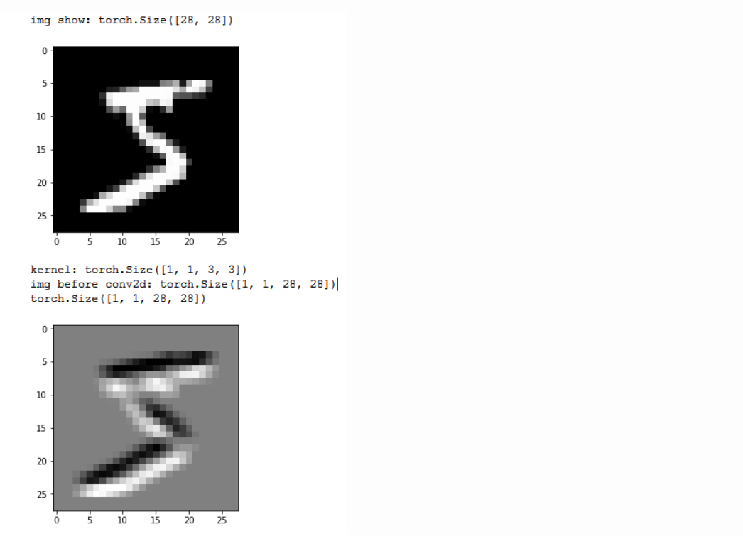
Check for the details on convolution.
Thanks to the E. Young we have the convolution-visualizer project on GitHub.
This interactive visualization demonstrates how various convolution parameters affect shapes and data dependencies between the input, weight and output matrices.
Convolution detects objects invariant to position since it can detects the features irrelevant to object location. This works for objects that are not rotated.
For instance, if you work on MNIST dataset you may notice all the images are centered.
The torch.nn.Conv2d model trained on MNIST will still work on brand new test images where cipher is outside of the center area. The model will still predict correct.
Linear layers won’t. If you train MNIST on torch.nn.Linear, it would detect purly objects (chipres) outside of the center area. This is because all MNIST images are centered.
nn.BatchNorm2d()
Batch normalization is the regularization technique for neural networks presented for the first time in 2015 in Batch Normalization: Accelerating Deep Network Training by Reducing Internal Covariate Shift paper.
Thanks to the batch norm for the first time the ImageNet exceeded the accuracy of human raters, and stepped the era where machine learning started to classify images better than humans (for the particular classification task).
This is why we say Batch Normalization is the milestone technique in the development of deep learning.
Essentially it shifts the distribution of the input to the z-distribution.
In PyTorch there are few things important for the batch norm (BN):
- BN is applied to every mini batch.
- For each feature $c_i$ (from C features) in the mini-batch (mb), BN computes the mean and variance of that feature.
- BN will then normalize each feature $c_i$, by subtracting the mean μ and will divide by standard deviation σ of that feature.
- If we have
affine=Falsewe will have what we stated so far. - If we have
affine=Truewe will have two more learnable parameters β and γ. γ is the slope (weight) and β is the intercept (bias) for the affine transformation. These parameters are learnable and initially they will be set to all zeros for β and all ones for γ.
Check for the details on Batch Norm.
nn.LayerNorm()
LayerNorm implementation principles are very similar to BatchNorm2d except instead averaging $\mu$ and $\sigma$ of a batch we do averaging over a feature for every feature.
torch.nn.LayerNorm(normalized_shape,
                   eps=1e-05,
                   elementwise_affine=True)
Great application of LayerNorm is for the Transformer model where it is used extensively.
nn.Dropout()
Example: Dropout effect
inp = torch.randn(2, 3)
print(inp)
m = nn.Dropout(p=0.5)
out = m(inp)
print(out)
Out:
tensor([[-2.1772,  0.7573, -0.0201],
        [ 0.9038,  0.3579,  0.5959]])
tensor([[-4.3543,  0.0000, -0.0402],
        [ 1.8076,  0.7157,  0.0000]])
Just to mark one very important thing. The number of zeros dropout creates will not always be 3 in the case of 6 elements tensor.
The probability p=0.5 is telling it should be 3 zeros on average, according to Bernoulli distribution. The Bernoulli distribution is a special case of the binomial distribution where a single trial is conducted.
However, it may be more or less zeros each time.
The nn.Dropout() is equivalent to torch.nn.functional.dropout() which is equivalent to torch.dropout().
One another important mark: Dropout works just in the training time. So the equivalent for the upper code in train time would be:
out = torch.dropout(inp, p=0.5, train=True)
Internally the to suppress the impact on zeros output is scaled by a factor of $\frac{1}{1-p}$. When not in training mode dropout is equivalent to identity function.
Custom Modules
What would be the simplest possible module you can create in PyTorch?
M0 minimal
import torch
import torch.nn as nn

class M0(nn.Module):
    def __init__(self):
        super().__init__()

    def forward(self)->None:
        print("empty module:forward")

# we create a module instance m1
m0 = M0()
m0()
# ??m0.__call__ # has forward() inside
Out:
empty module:forward
M1 Single Linear Layer
import torch
import torch.nn as nn

class M1(nn.Module):
    '''
    Single linear layer
    '''
    def __init__(self):
        super().__init__()
        self.l1 = nn.Linear(10,100)

    def forward(self,x)->None:
        print("M1:forward")
        x = self.l1(x)
        return x

# we create a module instance m1
m1 = M1()
print(m1)
x = torch.randn(1,10)
r = m1(x)
print(r.shape)
Out:
M1(
  (l1): Linear(in_features=10, out_features=100, bias=True)
)
M1:forward
torch.Size([1, 100])
M2 Combined Linear Layers
class M2(nn.Module):
    def __init__(self):
        super().__init__()
        self.l1 = nn.Linear(28*28, 10)
        self.l2 = nn.Linear(10, 10)

    def forward(self, x):
        x = x.reshape(-1, 28*28)
        x = F.relu(self.l1(x))
        x = F.relu(self.l2(x))
        return x
M2 Combined Conv2d Layers
class M3(nn.Module):
    def __init__(self):
        super().__init__()
        self.conv1 = nn.Conv2d(1, 16, kernel_size=3, stride=2, padding=1)
        self.conv2 = nn.Conv2d(16, 16, kernel_size=3, stride=2, padding=1)
        self.conv3 = nn.Conv2d(16, 10, kernel_size=3, stride=2, padding=1)

    def forward(self, xb):
        xb = xb.view(-1, 1, 28, 28)
        xb = F.relu(self.conv1(xb))
        xb = F.relu(self.conv2(xb))
        xb = F.relu(self.conv3(xb))
        xb = F.avg_pool2d(xb, 4)
        return xb.view(-1, xb.size(1))
Attention module
Attention module has been introduced with many papers so far. All started with the Transformer or Attention Is All You Need paper.
Key ideas of this paper are also used for GANs self attention.
I will start with explaining the self attention.
One implementation but not in PyTorch is in self attention gan repo.
Self attention key ideas:
- output dimension will be same as input dimension
If we provide an image the output will be the image equal in size.
- focus on a big picture
Convolution can provide good representation and understanding for the features that are close to each other. For instance, level of details from a dogs fer, but it “harder” mange the big picture. Sometimes dogs leg is missing.
To improve this, we need to have a mechanism that will understand the “big picture”. This effectively means to extract the features that are not close in the image.
For this reason we need to use the softmax function. This function selects just one from many values and it may be internally called “there can be only one”.
- query key value triplet
The attention is really based on the convolution learning triplet. Query self.query and key self.key are multiplied together. Once multiplied we pass the result to the softmax function to get beta tensor.
This passing trough the softmax function is equivalent to extracting the dominant features as we saw.
Then we multiply value self.value with the beta. This particular matrix multiplication may be called “extracting the similar features”. Then we multiply this with gamma vector parameter that we update as we learn. At the very start, gamma is vector of zeros.
This matrix multiplication is called matrix dot product. Multiplication is composed on vector inner products. This is how we catch similarities because inner product is biggest when cos.
We just need to provide a single thing to the self attention module: the number of input channels.
The self attention module works thanks to the conv1d in this case.
Example: Attention module
import torch
import torch.nn as nn
import torch.nn.functional as F
from torch.nn.utils import spectral_norm
class SelfAttention(nn.Module):
    "Self attention layer for `n_channels`."
    def __init__(self, n_channels):
        super().__init__()
        self.query = spectral_norm(
            nn.Conv1d(n_channels, 2, kernel_size=(1,), stride=(1,), bias=False))
        self.key = spectral_norm(
            nn.Conv1d(n_channels, 2, kernel_size=(1,), stride=(1,), bias=False))
        self.value = spectral_norm(
            nn.Conv1d(n_channels, 2*8, kernel_size=(1,), stride=(1,), bias=False))
        self.gamma = nn.Parameter(torch.tensor([0.]))


    def forward(self, x):
        size = x.size()
        print('size',size)
        x = x.view(*size[:2],-1) # (32, 16, 8, 8) ->  (32, 16, 64)
        print('x.shape:',x.shape)
        q,k,v = self.query(x),self.key(x),self.value(x)
        print('q:', q.shape)
        print('k:', k.shape)
        print('v:', v.shape)
        print('q.T:', q.transpose(1,2).shape)

        # beta is the super feature we try extract using the softmax
        beta = F.softmax(torch.bmm(q.transpose(1,2), k), dim=1) # query, key
        o = self.gamma * torch.bmm(v, beta) + x # value + original
        return o.view(*size).contiguous()

sa = SelfAttention(16)
print(sa)
x = torch.randn(32, 16, 8, 8)
print(x.shape)
out = sa(x)
print(out.shape)
Out:
SelfAttention(
  (query): Conv1d(16, 2, kernel_size=(1,), stride=(1,), bias=False)
  (key): Conv1d(16, 2, kernel_size=(1,), stride=(1,), bias=False)
  (value): Conv1d(16, 16, kernel_size=(1,), stride=(1,), bias=False)
)
torch.Size([32, 16, 8, 8])
size torch.Size([32, 16, 8, 8])
x.shape: torch.Size([32, 16, 64])
q: torch.Size([32, 2, 64])
k: torch.Size([32, 2, 64])
v: torch.Size([32, 16, 64])
q.T: torch.Size([32, 64, 2])
torch.Size([32, 16, 8, 8])
Iterate over modules
Several methods are there to iterate over modules.
modules()named_modules()children()named_children()
Ref: Children vs. named children example.
As you may see they provide the same feedback, thus named_children() may at certain time be more convenient because it provides you the module name.
Example: modules()
module = nn.Sequential(nn.Linear(2,2),
                  nn.ReLU(),
                  nn.Sequential(nn.Sigmoid(),
                  nn.ReLU()))

for m in module.modules():
    print(m)
Out:
Sequential(
  (0): Linear(in_features=2, out_features=2, bias=True)
  (1): ReLU()
  (2): Sequential(
    (0): Sigmoid()
    (1): ReLU()
  )
)
Linear(in_features=2, out_features=2, bias=True)
ReLU()
Sequential(
  (0): Sigmoid()
  (1): ReLU()
)
Sigmoid()
ReLU()
Example: named_modules()
module = nn.Sequential(nn.Linear(2,2),
                  nn.ReLU(),
                  nn.Sequential(nn.Sigmoid(),
                  nn.ReLU()))

for tuples in module.named_modules():
    print(tuples)
Out:
('', Sequential(
  (0): Linear(in_features=2, out_features=2, bias=True)
  (1): ReLU()
  (2): Sequential(
    (0): Sigmoid()
    (1): ReLU()
  )
))
('0', Linear(in_features=2, out_features=2, bias=True))
('1', ReLU())
('2', Sequential(
  (0): Sigmoid()
  (1): ReLU()
))
('2.0', Sigmoid())
('2.1', ReLU())
Example: children()
module = nn.Sequential(nn.Linear(2,2),
                  nn.ReLU(),
                  nn.Sequential(nn.Sigmoid(),
                  nn.ReLU()))

for m in module.children():
    print(m)
Out:
Linear(in_features=2, out_features=2, bias=True)
ReLU()
Sequential(
  (0): Sigmoid()
  (1): ReLU()
)
Example: named_children()
module = nn.Sequential(nn.Linear(2,2),
                  nn.ReLU(),
                  nn.Sequential(nn.Sigmoid(),
                  nn.ReLU()))

for tuples in module.named_children():
    print(tuples)
Out:
('0', Linear(in_features=2, out_features=2, bias=True))
('1', ReLU())
('2', Sequential(
  (0): Sigmoid()
  (1): ReLU()
))
How to check if model is on CUDA?
This code should do it:
import torch
import torchvision
model = torchvision.models.resnet18()
model.to('cuda')
next(model.parameters()).is_cuda
Out:
True
Note there is no is_cuda() method inside nn.Module. Also note model.to('cuda') is the same as model.cuda() and both are in-place.
On the other hand moving the data.to('cuda') is not inplace and you typically call:
data = data.to('cuda')
to move the data to CUDA.
…
tags: train & category: pytorch